Building a Transformer Model for Language Translation

 

The Transformer architecture, introduced in 2017, revolutionized sequence-to-sequence tasks like language translation by eliminating the need for recurrent neural networks. Instead, it relies on self-attention mechanisms to process input sequences. In this post, you’ll learn how to build a Transformer model from scratch. In particular, you will understand:

• How self-attention processes input sequences
• How transformer encoder and decoder work
• How to implement a complete translation system with a transformer

Kick-start your project with my book Building Transformer Models From Scratch with PyTorch. It provides self-study tutorials with working code.

Let’s get started.

Building a Transformer Model for Language Translation
Photo by Sorasak. Some rights reserved.

Overview

This post is divided into six parts; they are:

• Why Transformer is Better than Seq2Seq
• Data Preparation and Tokenization
• Design of a Transformer Model
• Building the Transformer Model
• Causal Mask and Padding Mask
• Training and Evaluation

Why Transformer is Better than Seq2Seq

Traditional seq2seq models with recurrent neural networks have two main limitations:

1. Sequential processing prevents parallelization
2. Limited ability to capture long-term dependencies since hidden states are overwritten whenever an element is processed

The Transformer architecture, introduced in the 2017 paper “Attention is All You Need”, overcomes these limitations. It can use the self-attention mechanism to capture dependencies between any position in the sequence. It can process the entire sequence in parallel. The sequence processing ability of a transformer model does not depend on recurrent connections.

Data Preparation and Tokenization

In this post, you will build a transformer model for translation, as this is the typical use case of a full transformer.

The dataset you will use is the English-French translation dataset from Anki, which contains pairs of English and French sentences. This is the same dataset you used in a previous post, and the preparation steps are similar.

French text contains accents and complex verb conjugations, requiring more sophisticated tokenization than simple word splitting. Byte-Pair Encoding (BPE) effectively handles these subword units and morphologically rich languages. It is also a good solution to handle unknown words.

Firstly, you would like to download the dataset and read it into memory. The dataset is a plain text file, and each line is an English and French sentence separated by a tab character. Below is how you can download and read the dataset:

import os import unicodedata import zipfile import requests   # Download dataset provided by Anki: https://www.manythings.org/anki/ with requests if not os.path.exists("fra-eng.zip"):     url = "http://storage.googleapis.com/download.tensorflow.org/data/fra-eng.zip"     response = requests.get(url)     with open("fra-eng.zip", "wb") as f:         f.write(response.content)   # Normalize text # each line of the file is in the format "<english>\t<french>" # We convert text to lowercase, normalize unicode (UFKC) def normalize(line):     """Normalize a line of text and split into two at the tab character"""     line = unicodedata.normalize("NFKC", line.strip().lower())     eng, fra = line.split("\t")     return eng.lower().strip(), fra.lower().strip()   text_pairs = [] with zipfile.ZipFile("fra-eng.zip", "r") as zip_ref:     for line in zip_ref.read("fra.txt").decode("utf-8").splitlines():         eng, fra = normalize(line)         text_pairs.append((eng, fra))

French sentences use Unicode characters, which can have multiple representation forms. We normalize the text to the “NFKC” form for consistent representation before processing. This is a good practice to make sure the text is “clean” so that the model can focus on the actual content of the text.

The translation pairs in text_pairs are pairs of strings of the complete sentences. You can use them to train a tokenizer in BPE, which you can use for the tokenization of future sentences:

import tokenizers   if os.path.exists("en_tokenizer.json") and os.path.exists("fr_tokenizer.json"):     en_tokenizer = tokenizers.Tokenizer.from_file("en_tokenizer.json")     fr_tokenizer = tokenizers.Tokenizer.from_file("fr_tokenizer.json") else:     en_tokenizer = tokenizers.Tokenizer(tokenizers.models.BPE())     fr_tokenizer = tokenizers.Tokenizer(tokenizers.models.BPE())       # Configure pre-tokenizer to split on whitespace and punctuation, add space at beginning of the sentence     en_tokenizer.pre_tokenizer = tokenizers.pre_tokenizers.ByteLevel(add_prefix_space=True)     fr_tokenizer.pre_tokenizer = tokenizers.pre_tokenizers.ByteLevel(add_prefix_space=True)       # Configure decoder: So that word boundary symbol "Ġ" will be removed     en_tokenizer.decoder = tokenizers.decoders.ByteLevel()     fr_tokenizer.decoder = tokenizers.decoders.ByteLevel()       # Train BPE for English and French using the same trainer     VOCAB_SIZE = 8000     trainer = tokenizers.trainers.BpeTrainer(         vocab_size=VOCAB_SIZE,         special_tokens=["[start]", "[end]", "[pad]"],         show_progress=True     )     en_tokenizer.train_from_iterator([x[0] for x in text_pairs], trainer=trainer)     fr_tokenizer.train_from_iterator([x[1] for x in text_pairs], trainer=trainer)       en_tokenizer.enable_padding(pad_id=en_tokenizer.token_to_id("[pad]"), pad_token="[pad]")     fr_tokenizer.enable_padding(pad_id=fr_tokenizer.token_to_id("[pad]"), pad_token="[pad]")       # Save the trained tokenizers     en_tokenizer.save("en_tokenizer.json", pretty=True)     fr_tokenizer.save("fr_tokenizer.json", pretty=True)

The code above uses the tokenizers library from Hugging Face to train the tokenizers. The trained tokenizers are saved as a JSON file for reuse. When you trained the tokenizers, you added three special tokens: [start], [end], and [pad]. These tokens are used to mark the beginning and end of the sentence and to pad the sequence to the same length. The tokenizers are set with enable_padding() such that when you use the tokenizer to process a string, padding tokens will be added. You will see how they are used in the following sections.

Below is an example of how you can use the tokenizer:

...   encoded = fr_tokenizer.encode("[start] " + fr_sample + " [end]") print(f"Original: {fr_sample}") print(f"Tokens: {encoded.tokens}") print(f"IDs: {encoded.ids}") print(f"Decoded: {fr_tokenizer.decode(encoded.ids)}")

The tokenizer not only splits the text into tokens, but also provides a way to encode the tokens into integer IDs. This is essential for the transformer model, as the model needs to process the input sequence as a sequence of numbers.

Design of a Transformer Model

A transformer combines an encoder and decoder. The encoder features multiple layers of self-attention and feed-forward networks, while the decoder incorporates cross-attention as well. The encoder processes the input sequence, and the decoder generates the output sequence, just like the case of the seq2seq model. Yet, there are many variations in a transformer model. Common architectural variations include:

• Positional Encoding: Provides positional information, as transformers process sequences in parallel. There are multiple strategies for passing the position of an element in the sequence to the model.
• Attention Mechanism: While scaled dot-product attention is standard, variations in its implementation, such as multi-head attention (MHA), multi-query attention (MQA), grouped query attention (GQA), and multi-head latent attention (MLA), exist at the model level. This is because each attention layer in a transformer model consists of multiple attention “heads” operating in parallel. These are the different ways to apply the input to the different heads.
• Feed-forward Network: This is a multi-layer perceptron network, but you can pick a different activation function or number of layers. In cases where a large model needs to handle a wide variety of inputs, a mixture-of-experts network can be used as an alternative to the feed-forward network.
• Layer Normalization: Layer norm or RMS norm should be applied between the attention and feed-forward networks. You can either use the “pre-norm” or “post-norm” with skip connections.
• Hyperparameters: For the same design, you can scale the model by adjusting the size of the hidden dimension, the number of heads/layers, the dropout rate, and the maximum sequence length that the model should support.

In this post, let’s use the following:

• Positional Encoding: Rotary Positional Encoding, with the maximum sequence length of 768
• Attention Mechanism: Grouped-Query Attention, with 8 query heads and 4 key-value heads
• Feed-forward Network: Two-layer SwiGLU, with a dimension of 512 in the hidden layer
• Layer Normalization: RMS Norm, in pre-norm
• Hidden dimension: 128
• Number of encoder and decoder layers: 4
• Dropout rate: 0.1

The transformer model to be built

The model you will build is illustrated as follows:

Building the Transformer Model

Various positional encoding methods and their implementations are covered in the previous post. For RoPE, this is the PyTorch implementation:

def rotate_half(x):     x1, x2 = x.chunk(2, dim=-1)     return torch.cat((-x2, x1), dim=-1)   def apply_rotary_pos_emb(x, cos, sin):     return (x * cos) + (rotate_half(x) * sin)   class RotaryPositionalEncoding(nn.Module):     def __init__(self, dim, max_seq_len=1024):         super().__init__()         N = 10000         inv_freq = 1. / (N ** (torch.arange(0, dim, 2).float() / dim))         position = torch.arange(max_seq_len).float()         inv_freq = torch.cat((inv_freq, inv_freq), dim=-1)         sinusoid_inp = torch.outer(position, inv_freq)         self.register_buffer("cos", sinusoid_inp.cos())         self.register_buffer("sin", sinusoid_inp.sin())       def forward(self, x, seq_len=None):         if seq_len is None:             seq_len = x.size(1)         cos = self.cos[:seq_len].view(1, seq_len, 1, -1)         sin = self.sin[:seq_len].view(1, seq_len, 1, -1)         return apply_rotary_pos_emb(x, cos, sin)

The rotary positional encoding changes the input vectors by multiplying every two elements of the vector by a 2×2 matrix of rotation:

ˆ𝐱𝑚=𝐑𝑚⁢𝐱𝑚=[cos⁡(𝑚⁢𝜃𝑖)−sin⁡(𝑚⁢𝜃𝑖)sin⁡(𝑚⁢𝜃𝑖)cos⁡(𝑚⁢𝜃𝑖)]⁢𝐱𝑚

For 𝐱𝑚 representing a pair (𝑖,𝑑/2 +𝑖) of elements in the vector at position 𝑚. The exact matrix used depends on the position 𝑚 of the vector in the sequence.

RoPE differs from the original Transformer’s sinusoidal positional encoding in that it is applied within the attention sublayer rather than outside it.

The attention you will use is the Grouped-Query Attention (GQA). PyTorch supports GQA, but in the attention sublayer, you should implement the projection of the query, key, and value. An implementation of GQA is covered in a previous post but below is an extended version that allows you to use it not only in self-attention, but also in cross-attention:

class GQA(nn.Module):     def __init__(self, hidden_dim, num_heads, num_kv_heads=None, dropout=0.1):         super().__init__()         self.num_heads = num_heads         self.num_kv_heads = num_kv_heads or num_heads         self.head_dim = hidden_dim // num_heads         self.num_groups = num_heads // num_kv_heads         self.dropout = dropout         self.q_proj = nn.Linear(hidden_dim, hidden_dim)         self.k_proj = nn.Linear(hidden_dim, hidden_dim)         self.v_proj = nn.Linear(hidden_dim, hidden_dim)         self.out_proj = nn.Linear(hidden_dim, hidden_dim)       def forward(self, q, k, v, mask=None, rope=None):         q_batch_size, q_seq_len, hidden_dim = q.shape         k_batch_size, k_seq_len, hidden_dim = k.shape         v_batch_size, v_seq_len, hidden_dim = v.shape           # projection         q = self.q_proj(q).view(q_batch_size, q_seq_len, -1, self.head_dim).transpose(1, 2)         k = self.k_proj(k).view(k_batch_size, k_seq_len, -1, self.head_dim).transpose(1, 2)         v = self.v_proj(v).view(v_batch_size, v_seq_len, -1, self.head_dim).transpose(1, 2)           # apply rotary positional encoding         if rope:             q = rope(q)             k = rope(k)           # compute grouped query attention         q = q.contiguous()         k = k.contiguous()         v = v.contiguous()         output = F.scaled_dot_product_attention(q, k, v,                                                 attn_mask=mask,                                                 dropout_p=self.dropout,                                                 enable_gqa=True)         output = output.transpose(1, 2).reshape(q_batch_size, q_seq_len, hidden_dim).contiguous()         output = self.out_proj(output)         return output

Note that in the forward() method of the GQA class, you can specify the positional encoding module in the rope argument. This makes the positional encoding optional. In PyTorch, for an optimized attention computation, the input tensors should be a contiguous block in memory. The line q = q.contiguous() is used to restructure the tensor if it is not already contiguous.

The feed-forward network you will use is the two-layer SwiGLU. The SwiGLU activation function is unique in that PyTorch does not support it, but it can be implemented using the SiLU activation. Below is an implementation of the feed-forward network using SwiGLU, from a previous post:

class SwiGLU(nn.Module):     def __init__(self, hidden_dim, intermediate_dim):         super().__init__()         self.gate = nn.Linear(hidden_dim, intermediate_dim)         self.up = nn.Linear(hidden_dim, intermediate_dim)         self.down = nn.Linear(intermediate_dim, hidden_dim)         self.act = nn.SiLU()       def forward(self, x):         x = self.act(self.gate(x)) * self.up(x)         x = self.down(x)         return x

With this, you can now build the encoder and decoder layers. The encoder layer is simpler, as it consists of a self-attention layer followed by a feed-forward network. However, you still need to implement skip connections and pre-norm using RMS norm. Below is the implementation of the encoder layer:

class EncoderLayer(nn.Module):     def __init__(self, hidden_dim, num_heads, num_kv_heads=None, dropout=0.1):         super().__init__()         self.self_attn = GQA(hidden_dim, num_heads, num_kv_heads, dropout)         self.mlp = SwiGLU(hidden_dim, 4 * hidden_dim)         self.norm1 = nn.RMSNorm(hidden_dim)         self.norm2 = nn.RMSNorm(hidden_dim)       def forward(self, x, mask=None, rope=None):         # self-attention sublayer         out = x         out = self.norm1(x)         out = self.self_attn(out, out, out, mask, rope)         x = out + x         # MLP sublayer         out = self.norm2(x)         out = self.mlp(out)         return out + x

The feed-forward network was implemented as SwiGLU module defined previously. You can see that the intermediate dimension is defined as 4 times the size of the hidden dimension. This is a common design in the industry, but you can experiment with a different ratio.

The decoder layer is more complex, as it consists of a self-attention layer, followed by a cross-attention layer, and finally a feed-forward network. The implementation is as follows:

class DecoderLayer(nn.Module):     def __init__(self, hidden_dim, num_heads, num_kv_heads=None, dropout=0.1):         super().__init__()         self.self_attn = GQA(hidden_dim, num_heads, num_kv_heads, dropout)         self.cross_attn = GQA(hidden_dim, num_heads, num_kv_heads, dropout)         self.mlp = SwiGLU(hidden_dim, 4 * hidden_dim)         self.norm1 = nn.RMSNorm(hidden_dim)         self.norm2 = nn.RMSNorm(hidden_dim)         self.norm3 = nn.RMSNorm(hidden_dim)       def forward(self, x, enc_out, mask=None, rope=None):         # self-attention sublayer         out = x         out = self.norm1(out)         out = self.self_attn(out, out, out, mask, rope)         x = out + x         # cross-attention sublayer         out = self.norm2(x)         out = self.cross_attn(out, enc_out, enc_out, None, rope)         x = out + x         # MLP sublayer         x = out + x         out = self.norm3(x)         out = self.mlp(out)         return out + x

You can see that both the self-attention and cross-attention sublayers are implemented using the GQA class. The difference is in how they are used in the forward() method. RoPE is applied to both, but the mask is only used in the self-attention sublayer.

The transformer model is built to connect encoders and decoders, but before passing on the sequence into the encoders or decoders, the input sequence of token IDs are first converted into embedding vectors. It is implemented as follows:

class Transformer(nn.Module):     def __init__(self, num_layers, num_heads, num_kv_heads, hidden_dim,                  max_seq_len, vocab_size_src, vocab_size_tgt, dropout=0.1):         super().__init__()         self.rope = RotaryPositionalEncoding(hidden_dim // num_heads, max_seq_len)         self.src_embedding = nn.Embedding(vocab_size_src, hidden_dim)         self.tgt_embedding = nn.Embedding(vocab_size_tgt, hidden_dim)         self.encoders = nn.ModuleList([             EncoderLayer(hidden_dim, num_heads, num_kv_heads, dropout) for _ in range(num_layers)         ])         self.decoders = nn.ModuleList([             DecoderLayer(hidden_dim, num_heads, num_kv_heads, dropout) for _ in range(num_layers)         ])         self.out = nn.Linear(hidden_dim, vocab_size_tgt)       def forward(self, src_ids, tgt_ids, src_mask=None, tgt_mask=None):         # Encoder         x = self.src_embedding(src_ids)         for encoder in self.encoders:             x = encoder(x, src_mask, self.rope)         enc_out = x         # Decoder         x = self.tgt_embedding(tgt_ids)         for decoder in self.decoders:             x = decoder(x, enc_out, tgt_mask, self.rope)         return self.out(x)

You can see that the Transformer class has numerous parameters in its constructor. This is because it serves as the entry point to create the entire model, which the Transformer class will initiate all sub-layers. This is a good design since you can define a Python dictionary as a model config. Below is an example of how you can create the model using the classes defined above:

model_config = {     "num_layers": 4,     "num_heads": 8,     "num_kv_heads": 4,     "hidden_dim": 128,     "max_seq_len": 768,     "vocab_size_src": len(en_tokenizer.get_vocab()),     "vocab_size_tgt": len(fr_tokenizer.get_vocab()),     "dropout": 0.1, } device = torch.device('cuda' if torch.cuda.is_available() else 'cpu') model = Transformer(**model_config).to(device)

Causal Mask and Padding Mask

The first step in training the model is to create a dataset object that can be used to iterate over the dataset in batches and a random order. In the previous section, you read the dataset into a list text_pairs. You also created the tokenizers for English and French. Now you can use the Dataset class from PyTorch to create a dataset object. Below is an implementation of the dataset object:

import torch from torch.utils.data import Dataset, DataLoader   class TranslationDataset(torch.utils.data.Dataset):     def __init__(self, text_pairs):         self.text_pairs = text_pairs       def __len__(self):         return len(self.text_pairs)       def __getitem__(self, idx):         eng, fra = self.text_pairs[idx]         return eng, "[start] " + fra + " [end]"     def collate_fn(batch):     en_str, fr_str = zip(*batch)     en_enc = en_tokenizer.encode_batch(en_str, add_special_tokens=True)     fr_enc = fr_tokenizer.encode_batch(fr_str, add_special_tokens=True)     en_ids = [enc.ids for enc in en_enc]     fr_ids = [enc.ids for enc in fr_enc]     return torch.tensor(en_ids), torch.tensor(fr_ids)   BATCH_SIZE = 32 dataset = TranslationDataset(text_pairs) dataloader = DataLoader(dataset, batch_size=BATCH_SIZE, shuffle=True, collate_fn=collate_fn)

You can try to print one sample from the dataset:

for en_ids, fr_ids in dataloader:     print(f"English: {en_ids}")     print(f"French: {fr_ids}")     break

The TranslationDataset class wraps text_pairs and adds [start] and [end] tokens to French sentences. The dataloader object provides batched, randomized samples after tokenization. The function collate_fn() handles tokenization and padding to ensure uniform sequence lengths within each batch.

For training, we use cross-entropy loss and Adam optimizer. The model employs teacher forcing technique, providing ground truth sequences to the decoder during training rather than reusing its own outputs. Note that in teacher forcing, the decoder should only see the first 𝑁 −1 tokens when it generates the 𝑁-th token.

A transformer is an architecture that can be parallelized. When you provide a sequence of length 𝑁 to the decoder, it can process all elements of the sequence in parallel and output a sequence of length 𝑁. Usually, we consider only the last element of this output sequence as the output. Alternatively, to save computation, you can use the last element of the input sequence as the “query” in the attention, while using the full input sequence as both the “key” and “value”.

If you are careful, you will notice that for a sequence of length 𝑁, you can train the model 𝑁 times. If the model can be parallelized, you can generate 𝑁 outputs in parallel for the same input sequence 𝑁. However, there is a problem: when the model generates output 𝑁, you want it to use only the sequence up to position 𝑁 −1, but not anything from position 𝑁 or later.

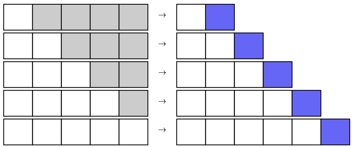
Causal prediction when you train a transformer: Iteratively you provide a longer sequence to the decoder (white squares). Each step, the decoder predict one additional output (blue squares). The gray squares are not provided to the model in the corresponding step.

To achieve this, use a causal mask. The causal mask is a square matrix of shape (𝑁,𝑁) for a sequence of length 𝑁. The causal mask nowadays is implemented as a triangular matrix, with all elements above the diagonal set to −∞ and the diagonal or below set to 0, like the following:

𝑀=⎡⎢ ⎢ ⎢ ⎢ ⎢⎣0−∞−∞⋯−∞00−∞⋯−∞000⋯−∞⋮⋮⋮⋱⋮000⋯0⎤⎥ ⎥ ⎥ ⎥ ⎥⎦

The causal mask is used in the decoder through the attention class GQA and in turn, used by the scaled_dot_product_attention() function in PyTorch. It will “mask out” the attention score at the position that is not allowed to attend to, i.e., the “future” positions, such that the softmax operation will set those positions to zero. The matrix 𝑀 illustrated above represents the “query” vertically and the “key” horizontally. The position of 0 in the matrix means the query can only attend to the key at a position no later than itself. Hence the name “causal”.

Causal mask is applied to the decoder’s self-attention, where the query and key are the same sequence. Hence, 𝑀 is a square matrix. You can create such a matrix in PyTorch as follows:

def create_causal_mask(seq_len, device):     mask = torch.triu(torch.full((seq_len, seq_len), float('-inf'), device=device), diagonal=1)     return mask

Besides the causal mask, you also want to skip the padding tokens in the sequence. Padding tokens are added when the sequences in a batch are not the same length. Since they are not supposed to carry any information, they should be excluded from the attention or loss computation at the output. The padding mask is also a square matrix for each sequence. The Python code to create one from a tensor of a batch of sequences is as follows:

def create_padding_mask(batch, padding_token_id):     batch_size, seq_len = batch.shape     device = batch.device     padded = torch.zeros_like(batch, device=device).float().masked_fill(batch == padding_token_id, float('-inf'))     mask = torch.zeros(batch_size, seq_len, seq_len, device=device) + padded[:,:,None] + padded[:,None,:]     return mask[:, None, :, :]

This code first creates a 2D tensor padded that matches the shape of the tensor batch. The tensor padded is zero everywhere except where the original tensor batch is equal to the padding token ID. Then a 3D tensor mask is created, with the shape of (𝑏⁢𝑎⁢𝑡⁢𝑐⁢ℎ𝑠⁡𝑖⁢𝑧⁢𝑒,𝑠⁢𝑒⁢𝑞𝑙⁢𝑒⁢𝑛,𝑠⁢𝑒⁢𝑞𝑙⁢𝑒⁢𝑛). The tensor mask is a batch of square matrices. In each square matrix, the rows and columns are set with padded in such a way that the positions corresponding to the padding tokens are set to −∞.

The function above uses the technique of dimension expansion in PyTorch. Indexing a tensor with None will add a new dimension at that position. It also uses the broadcasting feature of PyTorch to fill in mask with the padded tensor.

The padding mask created is of shape (batch_size, 1, seq_len, seq_len). The causal mask, however, is of shape (seq_len, seq_len). They can be broadcasted and added together when you apply self-attention.

Training and Evaluation

Now you can implement the training loop as follows:

N_EPOCHS = 60 LR = 0.005 WARMUP_STEPS = 1000 CLIP_NORM = 5.0   loss_fn = nn.CrossEntropyLoss(ignore_index=fr_tokenizer.token_to_id("[pad]"))   optimizer = optim.Adam(model.parameters(), lr=LR) warmup_scheduler = optim.lr_scheduler.LinearLR(     optimizer, start_factor=0.01, end_factor=1.0, total_iters=WARMUP_STEPS) cosine_scheduler = optim.lr_scheduler.CosineAnnealingLR(     optimizer, T_max=N_EPOCHS * len(dataloader) - WARMUP_STEPS, eta_min=0) scheduler = optim.lr_scheduler.SequentialLR(     optimizer, schedulers=[warmup_scheduler, cosine_scheduler], milestones=[WARMUP_STEPS])   for epoch in range(N_EPOCHS):     model.train()     epoch_loss = 0     for en_ids, fr_ids in dataloader:         # Move the "sentences" to device         en_ids = en_ids.to(device)         fr_ids = fr_ids.to(device)         # create source mask as padding mask, target mask as causal mask         src_mask = create_padding_mask(en_ids, en_tokenizer.token_to_id("[pad]"))         tgt_mask = create_causal_mask(fr_ids.shape[1], device).unsqueeze(0)         tgt_mask = tgt_mask + create_padding_mask(fr_ids, fr_tokenizer.token_to_id("[pad]"))         # zero the grad, then forward pass         optimizer.zero_grad()         outputs = model(en_ids, fr_ids, src_mask, tgt_mask)         # compute the loss: compare 3D logits to 2D targets         loss = loss_fn(outputs[:, :-1, :].reshape(-1, outputs.shape[-1]), fr_ids[:, 1:].reshape(-1))         loss.backward()         torch.nn.utils.clip_grad_norm_(model.parameters(), CLIP_NORM, error_if_nonfinite=False)         optimizer.step()         scheduler.step()         epoch_loss += loss.item()       print(f"Epoch {epoch+1}/{N_EPOCHS}; Avg loss {epoch_loss/len(dataloader)}; Latest loss {loss.item()}")

The training loop is implemented as a nested for-loop. Each epoch scans the entire dataset once. Each batch extracted from the dataset is used to create the masks. Then, the data and the mask are passed on to the model to generate the output. Then the loss is computed by comparing the output to the ground truth. The loss is backpropagated to update the model parameters.

The mask to use with the encoder is the padding mask from the source (English) sequence. The mask to use with the decoder is the causal mask plus the padding mask from the target (French) sequence. The gradient computed in the backward pass is clipped to mitigate the problem of exploding gradients.

While the training loop enables the model to learn to generate the target sequence, it is also beneficial to run an evaluation after each epoch to assess the model’s performance and save the best model. The evaluation is implemented as follows:

best_loss = float('inf') ...   model.eval() epoch_loss = 0 with torch.no_grad():     for en_ids, fr_ids in tqdm.tqdm(dataloader, desc="Evaluating"):         en_ids = en_ids.to(device)         fr_ids = fr_ids.to(device)         src_mask = create_padding_mask(en_ids, en_tokenizer.token_to_id("[pad]"))         tgt_mask = create_causal_mask(fr_ids.shape[1], device).unsqueeze(0) + create_padding_mask(fr_ids, fr_tokenizer.token_to_id("[pad]"))         outputs = model(en_ids, fr_ids, src_mask, tgt_mask)         loss = loss_fn(outputs[:, :-1, :].reshape(-1, outputs.shape[-1]), fr_ids[:, 1:].reshape(-1))         epoch_loss += loss.item() print(f"Eval loss: {epoch_loss/len(dataloader)}") if epoch_loss < best_loss:     best_loss = epoch_loss     torch.save(model.state_dict(), f"transformer-epoch-{epoch+1}.pth")

This evaluation reuses the same dataset as training because you do not have a separate test set. The code is similar to the training loop, except that you do not need the backward pass and run the model under torch.no_grad() context.

The loss is averaged over the entire dataset. The lowest loss is tracked by the variable best_loss. A copy of the model will be saved whenever the loss is improved.

A well-trained model should achieve an average loss of 0.1 or lower. Once the training is complete, your model is ready for use. Below is one example:

# Test for a few samples model.eval() N_SAMPLES = 5 MAX_LEN = 60 with torch.no_grad():     start_token = torch.tensor([fr_tokenizer.token_to_id("[start]")]).to(device)     for en, true_fr in random.sample(dataset.text_pairs, N_SAMPLES):         en_ids = torch.tensor(en_tokenizer.encode(en).ids).unsqueeze(0).to(device)           # get context from encoder         src_mask = create_padding_mask(en_ids, en_tokenizer.token_to_id("[pad]"))         x = model.src_embedding(en_ids)         for encoder in model.encoders:             x = encoder(x, src_mask, model.rope)         enc_out = x           # generate output from decoder         fr_ids = start_token.unsqueeze(0)         for _ in range(MAX_LEN):             tgt_mask = create_causal_mask(fr_ids.shape[1], device).unsqueeze(0)             tgt_mask = tgt_mask + create_padding_mask(fr_ids, fr_tokenizer.token_to_id("[pad]"))             x = model.tgt_embedding(fr_ids)             for decoder in model.decoders:                 x = decoder(x, enc_out, tgt_mask, model.rope)             outputs = model.out(x)               outputs = outputs.argmax(dim=-1)             fr_ids = torch.cat([fr_ids, outputs[:, -1:]], axis=-1)             if fr_ids[0, -1] == fr_tokenizer.token_to_id("[end]"):                 break           # Decode the predicted IDs         pred_fr = fr_tokenizer.decode(fr_ids[0].tolist())         print(f"English: {en}")         print(f"French: {true_fr}")         print(f"Predicted: {pred_fr}")         print()

This is more sophisticated than the training loop because you are not using the forward() method from the model, but using the encoder and decoder separately. You first use the encoder to get the context as enc_out. Then you started with fr_ids as the start token and iteratively generated the output from the decoder half of the transformer. Each step will extend fr_ids by one token. The generation will end when the end token is generated or when the maximum length is reached.

You can also use the forward() method from the model, but you will call the encoder with the same source sequence in each step. This is the unnecessary computation that was optimized in the above code. In reality, you may want to implement a method in the model class just for inference.

When you run the code above, you will see the following output:

English: are there any bananas? French: y a-t-il des bananes ? Predicted: y a-t-il des bananes ?   English: tom helped you, didn't he? French: tom t'a aidée, n'est-ce pas ? Predicted: tom vous a aidées, n'est-ce pas ?   English: i miss my parents. French: mes parents me manquent. Predicted: mes parents me manquent. j'ai manqué.   English: the game's almost over. French: la manche est presque terminée. Predicted: la manche est presque terminée.   English: turn left at the second traffic light. French: tourne au second feu à gauche ! Predicted: tournez au deuxième feu à gauche !

For completeness, the complete code is as follows:

# Transformer model implementation in PyTorch   import random import os import re import unicodedata import zipfile   import requests import torch import torch.nn as nn import torch.nn.functional as F import torch.optim as optim import tokenizers import tqdm     # # Data preparation #     # Download dataset provided by Anki: https://www.manythings.org/anki/ with requests if not os.path.exists("fra-eng.zip"):     url = "http://storage.googleapis.com/download.tensorflow.org/data/fra-eng.zip"     response = requests.get(url)     with open("fra-eng.zip", "wb") as f:         f.write(response.content)   # Normalize text # each line of the file is in the format "<english>\t<french>" # We convert text to lowercasee, normalize unicode (UFKC) def normalize(line):     """Normalize a line of text and split into two at the tab character"""     line = unicodedata.normalize("NFKC", line.strip().lower())     eng, fra = line.split("\t")     return eng.lower().strip(), fra.lower().strip()   text_pairs = [] with zipfile.ZipFile("fra-eng.zip", "r") as zip_ref:     for line in zip_ref.read("fra.txt").decode("utf-8").splitlines():         eng, fra = normalize(line)         text_pairs.append((eng, fra))   # # Tokenization with BPE #   if os.path.exists("en_tokenizer.json") and os.path.exists("fr_tokenizer.json"):     en_tokenizer = tokenizers.Tokenizer.from_file("en_tokenizer.json")     fr_tokenizer = tokenizers.Tokenizer.from_file("fr_tokenizer.json") else:     en_tokenizer = tokenizers.Tokenizer(tokenizers.models.BPE())     fr_tokenizer = tokenizers.Tokenizer(tokenizers.models.BPE())       # Configure pre-tokenizer to split on whitespace and punctuation, add space at beginning of the sentence     en_tokenizer.pre_tokenizer = tokenizers.pre_tokenizers.ByteLevel(add_prefix_space=True)     fr_tokenizer.pre_tokenizer = tokenizers.pre_tokenizers.ByteLevel(add_prefix_space=True)       # Configure decoder: So that word boundary symbol "Ġ" will be removed     en_tokenizer.decoder = tokenizers.decoders.ByteLevel()     fr_tokenizer.decoder = tokenizers.decoders.ByteLevel()       # Train BPE for English and French using the same trainer     VOCAB_SIZE = 8000     trainer = tokenizers.trainers.BpeTrainer(         vocab_size=VOCAB_SIZE,         special_tokens=["[start]", "[end]", "[pad]"],         show_progress=True     )     en_tokenizer.train_from_iterator([x[0] for x in text_pairs], trainer=trainer)     fr_tokenizer.train_from_iterator([x[1] for x in text_pairs], trainer=trainer)       en_tokenizer.enable_padding(pad_id=en_tokenizer.token_to_id("[pad]"), pad_token="[pad]")     fr_tokenizer.enable_padding(pad_id=fr_tokenizer.token_to_id("[pad]"), pad_token="[pad]")       # Save the trained tokenizers     en_tokenizer.save("en_tokenizer.json", pretty=True)     fr_tokenizer.save("fr_tokenizer.json", pretty=True)   # Test the tokenizer print("Sample tokenization:") en_sample, fr_sample = random.choice(text_pairs) encoded = en_tokenizer.encode(en_sample) print(f"Original: {en_sample}") print(f"Tokens: {encoded.tokens}") print(f"IDs: {encoded.ids}") print(f"Decoded: {en_tokenizer.decode(encoded.ids)}") print()   encoded = fr_tokenizer.encode("[start] " + fr_sample + " [end]") print(f"Original: {fr_sample}") print(f"Tokens: {encoded.tokens}") print(f"IDs: {encoded.ids}") print(f"Decoded: {fr_tokenizer.decode(encoded.ids)}") print()     # # Create PyTorch dataset for the BPE-encoded translation pairs #   class TranslationDataset(torch.utils.data.Dataset):     def __init__(self, text_pairs, en_tokenizer, fr_tokenizer):         self.text_pairs = text_pairs       def __len__(self):         return len(self.text_pairs)       def __getitem__(self, idx):         eng, fra = self.text_pairs[idx]         return eng, "[start] " + fra + " [end]"     def collate_fn(batch):     en_str, fr_str = zip(*batch)     en_enc = en_tokenizer.encode_batch(en_str, add_special_tokens=True)     fr_enc = fr_tokenizer.encode_batch(fr_str, add_special_tokens=True)     en_ids = [enc.ids for enc in en_enc]     fr_ids = [enc.ids for enc in fr_enc]     return torch.tensor(en_ids), torch.tensor(fr_ids)     BATCH_SIZE = 32 dataset = TranslationDataset(text_pairs, en_tokenizer, fr_tokenizer) dataloader = torch.utils.data.DataLoader(dataset, batch_size=BATCH_SIZE, shuffle=True, collate_fn=collate_fn)     # Test the dataset for en_ids, fr_ids in dataloader:     print(f"English: {en_ids}")     print(f"French: {fr_ids}")     break     # # Transformer model components #   def rotate_half(x):     x1, x2 = x.chunk(2, dim=-1)     return torch.cat((-x2, x1), dim=-1)     def apply_rotary_pos_emb(x, cos, sin):     return (x * cos) + (rotate_half(x) * sin)     class RotaryPositionalEncoding(nn.Module):     def __init__(self, dim, max_seq_len=1024):         super().__init__()         N = 10000         inv_freq = 1. / (N ** (torch.arange(0, dim, 2).float() / dim))         position = torch.arange(max_seq_len).float()         inv_freq = torch.cat((inv_freq, inv_freq), dim=-1)         sinusoid_inp = torch.outer(position, inv_freq)         self.register_buffer("cos", sinusoid_inp.cos())         self.register_buffer("sin", sinusoid_inp.sin())       def forward(self, x, seq_len=None):         if seq_len is None:             seq_len = x.size(1)         cos = self.cos[:seq_len].view(1, seq_len, 1, -1)         sin = self.sin[:seq_len].view(1, seq_len, 1, -1)         return apply_rotary_pos_emb(x, cos, sin)     class SwiGLU(nn.Module):     def __init__(self, hidden_dim, intermediate_dim):         super().__init__()         self.gate = nn.Linear(hidden_dim, intermediate_dim)         self.up = nn.Linear(hidden_dim, intermediate_dim)         self.down = nn.Linear(intermediate_dim, hidden_dim)         self.act = nn.SiLU()       def forward(self, x):         x = self.act(self.gate(x)) * self.up(x)         x = self.down(x)         return x     class GQA(nn.Module):     def __init__(self, hidden_dim, num_heads, num_kv_heads=None, dropout=0.1):         super().__init__()         self.num_heads = num_heads         self.num_kv_heads = num_kv_heads or num_heads         self.head_dim = hidden_dim // num_heads         self.num_groups = num_heads // num_kv_heads         self.dropout = dropout         self.q_proj = nn.Linear(hidden_dim, hidden_dim)         self.k_proj = nn.Linear(hidden_dim, hidden_dim)         self.v_proj = nn.Linear(hidden_dim, hidden_dim)         self.out_proj = nn.Linear(hidden_dim, hidden_dim)       def forward(self, q, k, v, mask=None, rope=None):         q_batch_size, q_seq_len, hidden_dim = q.shape         k_batch_size, k_seq_len, hidden_dim = k.shape         v_batch_size, v_seq_len, hidden_dim = v.shape           # projection         q = self.q_proj(q).view(q_batch_size, q_seq_len, -1, self.head_dim).transpose(1, 2)         k = self.k_proj(k).view(k_batch_size, k_seq_len, -1, self.head_dim).transpose(1, 2)         v = self.v_proj(v).view(v_batch_size, v_seq_len, -1, self.head_dim).transpose(1, 2)           # apply rotary positional encoding         if rope:             q = rope(q)             k = rope(k)           # compute grouped query attention         q = q.contiguous()         k = k.contiguous()         v = v.contiguous()         output = F.scaled_dot_product_attention(q, k, v,                                                 attn_mask=mask,                                                 dropout_p=self.dropout,                                                 enable_gqa=True)         output = output.transpose(1, 2).reshape(q_batch_size, q_seq_len, hidden_dim).contiguous()         output = self.out_proj(output)         return output     class EncoderLayer(nn.Module):     def __init__(self, hidden_dim, num_heads, num_kv_heads=None, dropout=0.1):         super().__init__()         self.self_attn = GQA(hidden_dim, num_heads, num_kv_heads, dropout)         self.mlp = SwiGLU(hidden_dim, 4 * hidden_dim)         self.norm1 = nn.RMSNorm(hidden_dim)         self.norm2 = nn.RMSNorm(hidden_dim)       def forward(self, x, mask=None, rope=None):         # self-attention sublayer         out = x         out = self.norm1(x)         out = self.self_attn(out, out, out, mask, rope)         x = out + x         # MLP sublayer         out = self.norm2(x)         out = self.mlp(out)         return out + x     class DecoderLayer(nn.Module):     def __init__(self, hidden_dim, num_heads, num_kv_heads=None, dropout=0.1):         super().__init__()         self.self_attn = GQA(hidden_dim, num_heads, num_kv_heads, dropout)         self.cross_attn = GQA(hidden_dim, num_heads, num_kv_heads, dropout)         self.mlp = SwiGLU(hidden_dim, 4 * hidden_dim)         self.norm1 = nn.RMSNorm(hidden_dim)         self.norm2 = nn.RMSNorm(hidden_dim)         self.norm3 = nn.RMSNorm(hidden_dim)       def forward(self, x, enc_out, mask=None, rope=None):         # self-attention sublayer         out = x         out = self.norm1(out)         out = self.self_attn(out, out, out, mask, rope)         x = out + x         # cross-attention sublayer         out = self.norm2(x)         out = self.cross_attn(out, enc_out, enc_out, None, rope)         x = out + x         # MLP sublayer         x = out + x         out = self.norm3(x)         out = self.mlp(out)         return out + x     class Transformer(nn.Module):     def __init__(self, num_layers, num_heads, num_kv_heads, hidden_dim,                  max_seq_len, vocab_size_src, vocab_size_tgt, dropout=0.1):         super().__init__()         self.rope = RotaryPositionalEncoding(hidden_dim // num_heads, max_seq_len)         self.src_embedding = nn.Embedding(vocab_size_src, hidden_dim)         self.tgt_embedding = nn.Embedding(vocab_size_tgt, hidden_dim)         self.encoders = nn.ModuleList([             EncoderLayer(hidden_dim, num_heads, num_kv_heads, dropout) for _ in range(num_layers)         ])         self.decoders = nn.ModuleList([             DecoderLayer(hidden_dim, num_heads, num_kv_heads, dropout) for _ in range(num_layers)         ])         self.out = nn.Linear(hidden_dim, vocab_size_tgt)       def forward(self, src_ids, tgt_ids, src_mask=None, tgt_mask=None):         # Encoder         x = self.src_embedding(src_ids)         for encoder in self.encoders:             x = encoder(x, src_mask, self.rope)         enc_out = x         # Decoder         x = self.tgt_embedding(tgt_ids)         for decoder in self.decoders:             x = decoder(x, enc_out, tgt_mask, self.rope)         return self.out(x)     model_config = {     "num_layers": 4,     "num_heads": 8,     "num_kv_heads": 4,     "hidden_dim": 128,     "max_seq_len": 768,     "vocab_size_src": len(en_tokenizer.get_vocab()),     "vocab_size_tgt": len(fr_tokenizer.get_vocab()),     "dropout": 0.1, } device = torch.device('cuda' if torch.cuda.is_available() else 'cpu') model = Transformer(**model_config).to(device) print(model)   # Training   print("Model created with:") print(f"  Input vocabulary size: {model_config['vocab_size_src']}") print(f"  Output vocabulary size: {model_config['vocab_size_tgt']}") print(f"  Number of layers: {model_config['num_layers']}") print(f"  Number of heads: {model_config['num_heads']}") print(f"  Number of KV heads: {model_config['num_kv_heads']}") print(f"  Hidden dimension: {model_config['hidden_dim']}") print(f"  Max sequence length: {model_config['max_seq_len']}") print(f"  Dropout: {model_config['dropout']}") print(f"  Total parameters: {sum(p.numel() for p in model.parameters() if p.requires_grad)}")   def create_causal_mask(seq_len, device):     """     Create a causal mask for autoregressive attention.       Args:         seq_len: Length of the sequence       Returns:         Causal mask of shape (seq_len, seq_len)     """     mask = torch.triu(torch.full((seq_len, seq_len), float('-inf'), device=device), diagonal=1)     return mask     def create_padding_mask(batch, padding_token_id):     """     Create a padding mask for a batch of sequences.       Args:         batch: Batch of sequences, shape (batch_size, seq_len)         padding_token_id: ID of the padding token       Returns:         Padding mask of shape (batch_size, seq_len, seq_len)     """     batch_size, seq_len = batch.shape     device = batch.device     padded = torch.zeros_like(batch, device=device).float().masked_fill(batch == padding_token_id, float('-inf'))     mask = torch.zeros(batch_size, seq_len, seq_len, device=device) + padded[:,:,None] + padded[:,None,:]     return mask[:, None, :, :]     # Train unless model.pth exists loss_fn = nn.CrossEntropyLoss(ignore_index=fr_tokenizer.token_to_id("[pad]")) if os.path.exists("transformer.pth"):     model.load_state_dict(torch.load("transformer.pth")) else:     N_EPOCHS = 60     LR = 0.005     WARMUP_STEPS = 1000     CLIP_NORM = 5.0     best_loss = float('inf')     optimizer = optim.Adam(model.parameters(), lr=LR)     warmup_scheduler = optim.lr_scheduler.LinearLR(optimizer, start_factor=0.01, end_factor=1.0, total_iters=WARMUP_STEPS)     cosine_scheduler = optim.lr_scheduler.CosineAnnealingLR(optimizer, T_max=N_EPOCHS * len(dataloader) - WARMUP_STEPS, eta_min=0)     scheduler = optim.lr_scheduler.SequentialLR(optimizer, schedulers=[warmup_scheduler, cosine_scheduler], milestones=[WARMUP_STEPS])     print(f"Training for {N_EPOCHS} epochs with {len(dataloader)} steps per epoch")       for epoch in range(N_EPOCHS):         model.train()         epoch_loss = 0         for en_ids, fr_ids in tqdm.tqdm(dataloader, desc="Training"):             # Move the "sentences" to device             en_ids = en_ids.to(device)             fr_ids = fr_ids.to(device)             # create source mask as padding mask, target mask as causal mask             src_mask = create_padding_mask(en_ids, en_tokenizer.token_to_id("[pad]"))             tgt_mask = create_causal_mask(fr_ids.shape[1], device).unsqueeze(0) + create_padding_mask(fr_ids, fr_tokenizer.token_to_id("[pad]"))             # zero the grad, then forward pass             optimizer.zero_grad()             outputs = model(en_ids, fr_ids, src_mask, tgt_mask)             # compute the loss: compare 3D logits to 2D targets             loss = loss_fn(outputs[:, :-1, :].reshape(-1, outputs.shape[-1]), fr_ids[:, 1:].reshape(-1))             loss.backward()             if CLIP_NORM:                 torch.nn.utils.clip_grad_norm_(model.parameters(), CLIP_NORM, error_if_nonfinite=False)             optimizer.step()             scheduler.step()             epoch_loss += loss.item()         print(f"Epoch {epoch+1}/{N_EPOCHS}; Avg loss {epoch_loss/len(dataloader)}; Latest loss {loss.item()}")         # Test         model.eval()         epoch_loss = 0         with torch.no_grad():             for en_ids, fr_ids in tqdm.tqdm(dataloader, desc="Evaluating"):                 en_ids = en_ids.to(device)                 fr_ids = fr_ids.to(device)                 src_mask = create_padding_mask(en_ids, en_tokenizer.token_to_id("[pad]"))                 tgt_mask = create_causal_mask(fr_ids.shape[1], device).unsqueeze(0) + create_padding_mask(fr_ids, fr_tokenizer.token_to_id("[pad]"))                 outputs = model(en_ids, fr_ids, src_mask, tgt_mask)                 loss = loss_fn(outputs[:, :-1, :].reshape(-1, outputs.shape[-1]), fr_ids[:, 1:].reshape(-1))                 epoch_loss += loss.item()         print(f"Eval loss: {epoch_loss/len(dataloader)}")         if epoch_loss < best_loss:             best_loss = epoch_loss             torch.save(model.state_dict(), f"transformer-epoch-{epoch+1}.pth")       # Save the final model after training     torch.save(model.state_dict(), "transformer.pth")   # Test for a few samples model.eval() N_SAMPLES = 5 MAX_LEN = 60 with torch.no_grad():     start_token = torch.tensor([fr_tokenizer.token_to_id("[start]")]).to(device)     for en, true_fr in random.sample(dataset.text_pairs, N_SAMPLES):         en_ids = torch.tensor(en_tokenizer.encode(en).ids).unsqueeze(0).to(device)           # get context from encoder         src_mask = create_padding_mask(en_ids, en_tokenizer.token_to_id("[pad]"))         x = model.src_embedding(en_ids)         for encoder in model.encoders:             x = encoder(x, src_mask, model.rope)         enc_out = x           # generate output from decoder         fr_ids = start_token.unsqueeze(0)         for _ in range(MAX_LEN):             tgt_mask = create_causal_mask(fr_ids.shape[1], device).unsqueeze(0)             tgt_mask = tgt_mask + create_padding_mask(fr_ids, fr_tokenizer.token_to_id("[pad]"))             x = model.tgt_embedding(fr_ids)             for decoder in model.decoders:                 x = decoder(x, enc_out, tgt_mask, model.rope)             outputs = model.out(x)               outputs = outputs.argmax(dim=-1)             fr_ids = torch.cat([fr_ids, outputs[:, -1:]], axis=-1)             if fr_ids[0, -1] == fr_tokenizer.token_to_id("[end]"):                 break           # Decode the predicted IDs         pred_fr = fr_tokenizer.decode(fr_ids[0].tolist())         print(f"English: {en}")         print(f"French: {true_fr}")         print(f"Predicted: {pred_fr}")         print()

Further Readings

Below are some references that you can use to learn more about the transformer model:

• The Illustrated Transformer
• The Annotated Transformer
• Attention is All You Need

Summary

In this post, you built and trained a complete Transformer model for English-French translation. In particular, you learned:

• Transformers replace recurrent layers with parallel processing via self-attention
• Various architectural choices affect model design and performance
• How to create the core components, including self-attention, cross-attention, and positional encoding
• How to train the model with masks and teacher forcing

While this implementation is modest in scale, it contains all the fundamental elements found in large language models.