It can be challenging to develop a neural network predictive model for a new dataset.
One approach is to first inspect the dataset and develop ideas for what models might work, then explore the learning dynamics of simple models on the dataset, then finally develop and tune a model for the dataset with a robust test harness.
This process can be used to develop effective neural network models for classification and regression predictive modeling problems.
In this tutorial, you will discover how to develop a Multilayer Perceptron neural network model for the banknote binary classification dataset.
After completing this tutorial, you will know:
- How to load and summarize the banknote dataset and use the results to suggest data preparations and model configurations to use.
- How to explore the learning dynamics of simple MLP models on the dataset.
- How to develop robust estimates of model performance, tune model performance and make predictions on new data.
Let’s get started.
- Update Oct/2021: Deprecated predict_classes() syntax

Develop a Neural Network for Banknote Authentication
Photo by Lenny K Photography, some rights reserved.
Tutorial Overview
This tutorial is divided into 4 parts; they are:
- Banknote Classification Dataset
- Neural Network Learning Dynamics
- Robust Model Evaluation
- Final Model and Make Predictions
Banknote Classification Dataset
The first step is to define and explore the dataset.
We will be working with the “Banknote” standard binary classification dataset.
The banknote dataset involves predicting whether a given banknote is authentic given a number of measures taken from a photograph.
The dataset contains 1,372 rows with 5 numeric variables. It is a classification problem with two classes (binary classification).
Below provides a list of the five variables in the dataset.
- variance of Wavelet Transformed image (continuous).
- skewness of Wavelet Transformed image (continuous).
- kurtosis of Wavelet Transformed image (continuous).
- entropy of image (continuous).
- class (integer).
Below is a sample of the first 5 rows of the dataset
| 3.6216,8.6661,-2.8073,-0.44699,0 4.5459,8.1674,-2.4586,-1.4621,0 3.866,-2.6383,1.9242,0.10645,0 3.4566,9.5228,-4.0112,-3.5944,0 0.32924,-4.4552,4.5718,-0.9888,0 4.3684,9.6718,-3.9606,-3.1625,0 ... |
You can learn more about the dataset here:
We can load the dataset as a pandas DataFrame directly from the URL; for example:
| # load the banknote dataset and summarize the shape from pandas import read_csv # define the location of the dataset url = 'https://raw.githubusercontent.com/jbrownlee/Datasets/master/banknote_authentication.csv' # load the dataset df = read_csv(url, header=None) # summarize shape print(df.shape) |
Running the example loads the dataset directly from the URL and reports the shape of the dataset.
In this case, we can confirm that the dataset has 5 variables (4 input and one output) and that the dataset has 1,372 rows of data.
This is not many rows of data for a neural network and suggests that a small network, perhaps with regularization, would be appropriate.
It also suggests that using k-fold cross-validation would be a good idea given that it will give a more reliable estimate of model performance than a train/test split and because a single model will fit in seconds instead of hours or days with the largest datasets.
Next, we can learn more about the dataset by looking at summary statistics and a plot of the data.
| # show summary statistics and plots of the banknote dataset from pandas import read_csv from matplotlib import pyplot # define the location of the dataset url = 'https://raw.githubusercontent.com/jbrownlee/Datasets/master/banknote_authentication.csv' # load the dataset df = read_csv(url, header=None) # show summary statistics print(df.describe()) # plot histograms df.hist() pyplot.show() |
Running the example first loads the data before and then prints summary statistics for each variable.
We can see that values vary with different means and standard deviations, perhaps some normalization or standardization would be required prior to modeling.
| 0 1 2 3 4 count 1372.000000 1372.000000 1372.000000 1372.000000 1372.000000 mean 0.433735 1.922353 1.397627 -1.191657 0.444606 std 2.842763 5.869047 4.310030 2.101013 0.497103 min -7.042100 -13.773100 -5.286100 -8.548200 0.000000 25% -1.773000 -1.708200 -1.574975 -2.413450 0.000000 50% 0.496180 2.319650 0.616630 -0.586650 0.000000 75% 2.821475 6.814625 3.179250 0.394810 1.000000 max 6.824800 12.951600 17.927400 2.449500 1.000000 |
A histogram plot is then created for each variable.
We can see that perhaps the first two variables have a Gaussian-like distribution and the next two input variables may have a skewed Gaussian distribution or an exponential distribution.
We may have some benefit in using a power transform on each variable in order to make the probability distribution less skewed which will likely improve model performance.
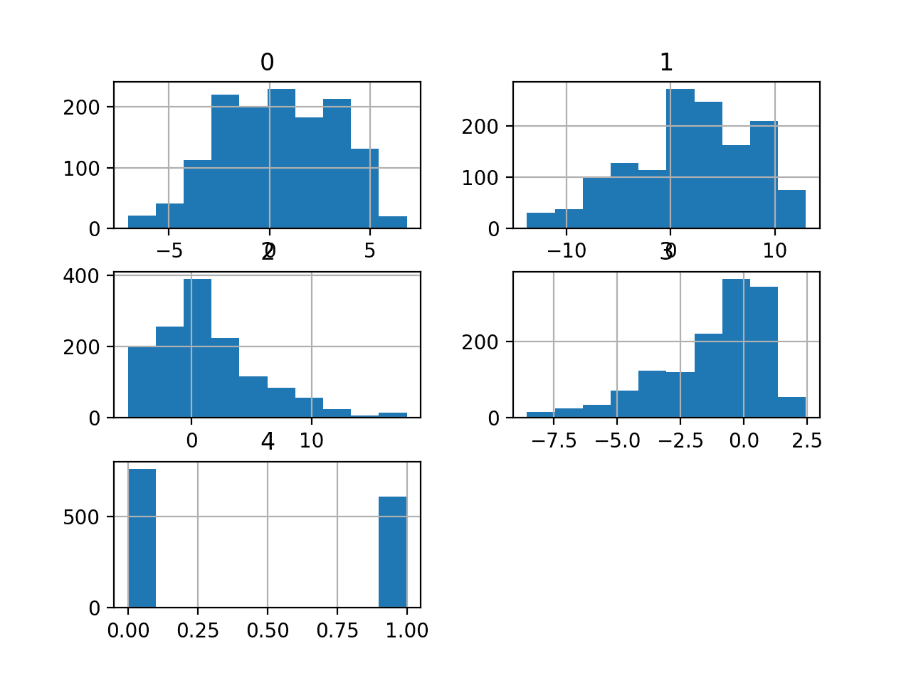
Histograms of the Banknote Classification Dataset
Now that we are familiar with the dataset, let’s explore how we might develop a neural network model.
Neural Network Learning Dynamics
We will develop a Multilayer Perceptron (MLP) model for the dataset using TensorFlow.
We cannot know what model architecture of learning hyperparameters would be good or best for this dataset, so we must experiment and discover what works well.
Given that the dataset is small, a small batch size is probably a good idea, e.g. 16 or 32 rows. Using the Adam version of stochastic gradient descent is a good idea when getting started as it will automatically adapt the learning rate and works well on most datasets.
Before we evaluate models in earnest, it is a good idea to review the learning dynamics and tune the model architecture and learning configuration until we have stable learning dynamics, then look at getting the most out of the model.
We can do this by using a simple train/test split of the data and review plots of the learning curves. This will help us see if we are over-learning or under-learning; then we can adapt the configuration accordingly.
First, we must ensure all input variables are floating-point values and encode the target label as integer values 0 and 1.
| ... # ensure all data are floating point values X = X.astype('float32') # encode strings to integer y = LabelEncoder().fit_transform(y) |
Next, we can split the dataset into input and output variables, then into 67/33 train and test sets.
| ... # split into input and output columns X, y = df.values[:, :-1], df.values[:, -1] # split into train and test datasets X_train, X_test, y_train, y_test = train_test_split(X, y, test_size=0.33) |
We can define a minimal MLP model. In this case, we will use one hidden layer with 10 nodes and one output layer (chosen arbitrarily). We will use the ReLU activation function in the hidden layer and the “he_normal” weight initialization, as together, they are a good practice.
The output of the model is a sigmoid activation for binary classification and we will minimize binary cross-entropy loss.
| ... # determine the number of input features n_features = X.shape[1] # define model model = Sequential() model.add(Dense(10, activation='relu', kernel_initializer='he_normal', input_shape=(n_features,))) model.add(Dense(1, activation='sigmoid')) # compile the model model.compile(optimizer='adam', loss='binary_crossentropy') |
We will fit the model for 50 training epochs (chosen arbitrarily) with a batch size of 32 because it is a small dataset.
We are fitting the model on raw data, which we think might be a good idea, but it is an important starting point.
| ... # fit the model history = model.fit(X_train, y_train, epochs=50, batch_size=32, verbose=0, validation_data=(X_test,y_test)) |
At the end of training, we will evaluate the model’s performance on the test dataset and report performance as the classification accuracy.
| ... # predict test set and convert to class label ypred = model.predict(X_test) yhat = (ypred > 0.5).flatten().astype(int) # evaluate predictions score = accuracy_score(y_test, yhat) print('Accuracy: %.3f' % score) |
Finally, we will plot learning curves of the cross-entropy loss on the train and test sets during training.
| ... # plot learning curves pyplot.title('Learning Curves') pyplot.xlabel('Epoch') pyplot.ylabel('Cross Entropy') pyplot.plot(history.history['loss'], label='train') pyplot.plot(history.history['val_loss'], label='val') pyplot.legend() pyplot.show() |
Tying this all together, the complete example of evaluating our first MLP on the banknote dataset is listed below.
1 2 3 4 5 6 7 8 9 10 11 12 13 14 15 16 17 18 19 20 21 22 23 24 25 26 27 28 29 30 31 32 33 34 35 36 37 38 39 40 41 42 43 | # fit a simple mlp model on the banknote and review learning curves from pandas import read_csv from sklearn.model_selection import train_test_split from sklearn.preprocessing import LabelEncoder from sklearn.metrics import accuracy_score from tensorflow.keras import Sequential from tensorflow.keras.layers import Dense from matplotlib import pyplot # load the dataset path = 'https://raw.githubusercontent.com/jbrownlee/Datasets/master/banknote_authentication.csv' df = read_csv(path, header=None) # split into input and output columns X, y = df.values[:, :-1], df.values[:, -1] # ensure all data are floating point values X = X.astype('float32') # encode strings to integer y = LabelEncoder().fit_transform(y) # split into train and test datasets X_train, X_test, y_train, y_test = train_test_split(X, y, test_size=0.33) # determine the number of input features n_features = X.shape[1] # define model model = Sequential() model.add(Dense(10, activation='relu', kernel_initializer='he_normal', input_shape=(n_features,))) model.add(Dense(1, activation='sigmoid')) # compile the model model.compile(optimizer='adam', loss='binary_crossentropy') # fit the model history = model.fit(X_train, y_train, epochs=50, batch_size=32, verbose=0, validation_data=(X_test,y_test)) # predict test set and convert to class label ypred = model.predict(X_test) yhat = (ypred > 0.5).flatten().astype(int) # evaluate predictions score = accuracy_score(y_test, yhat) print('Accuracy: %.3f' % score) # plot learning curves pyplot.title('Learning Curves') pyplot.xlabel('Epoch') pyplot.ylabel('Cross Entropy') pyplot.plot(history.history['loss'], label='train') pyplot.plot(history.history['val_loss'], label='val') pyplot.legend() pyplot.show() |
Running the example first fits the model on the training dataset, then reports the classification accuracy on the test dataset.
Note: Your results may vary given the stochastic nature of the algorithm or evaluation procedure, or differences in numerical precision. Consider running the example a few times and compare the average outcome.
In this case, we can see that the model achieved great or perfect accuracy of 100% percent. This might suggest that the prediction problem is easy and/or that neural networks are a good fit for the problem.
Line plots of the loss on the train and test sets are then created.
We can see that the model appears to converge well and does not show any signs of overfitting or underfitting.
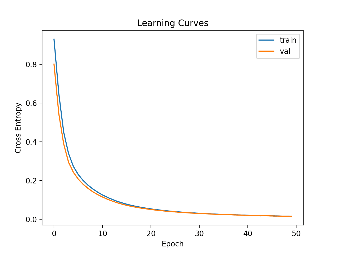
Learning Curves of Simple Multilayer Perceptron on Banknote Dataset
We did amazingly well on our first try.
Now that we have some idea of the learning dynamics for a simple MLP model on the dataset, we can look at developing a more robust evaluation of model performance on the dataset.
Robust Model Evaluation
The k-fold cross-validation procedure can provide a more reliable estimate of MLP performance, although it can be very slow.
This is because k models must be fit and evaluated. This is not a problem when the dataset size is small, such as the banknote dataset.
We can use the StratifiedKFold class and enumerate each fold manually, fit the model, evaluate it, and then report the mean of the evaluation scores at the end of the procedure.
| ... # prepare cross validation kfold = KFold(10) # enumerate splits scores = list() for train_ix, test_ix in kfold.split(X, y): # fit and evaluate the model... ... ... # summarize all scores print('Mean Accuracy: %.3f (%.3f)' % (mean(scores), std(scores))) |
We can use this framework to develop a reliable estimate of MLP model performance with our base configuration, and even with a range of different data preparations, model architectures, and learning configurations.
It is important that we first developed an understanding of the learning dynamics of the model on the dataset in the previous section before using k-fold cross-validation to estimate the performance. If we started to tune the model directly, we might get good results, but if not, we might have no idea of why, e.g. that the model was over or under fitting.
If we make large changes to the model again, it is a good idea to go back and confirm that the model is converging appropriately.
The complete example of this framework to evaluate the base MLP model from the previous section is listed below.
1 2 3 4 5 6 7 8 9 10 11 12 13 14 15 16 17 18 19 20 21 22 23 24 25 26 27 28 29 30 31 32 33 34 35 36 37 38 39 40 41 42 43 44 45 | # k-fold cross-validation of base model for the banknote dataset from numpy import mean from numpy import std from pandas import read_csv from sklearn.model_selection import StratifiedKFold from sklearn.preprocessing import LabelEncoder from sklearn.metrics import accuracy_score from tensorflow.keras import Sequential from tensorflow.keras.layers import Dense from matplotlib import pyplot # load the dataset path = 'https://raw.githubusercontent.com/jbrownlee/Datasets/master/banknote_authentication.csv' df = read_csv(path, header=None) # split into input and output columns X, y = df.values[:, :-1], df.values[:, -1] # ensure all data are floating point values X = X.astype('float32') # encode strings to integer y = LabelEncoder().fit_transform(y) # prepare cross validation kfold = StratifiedKFold(10) # enumerate splits scores = list() for train_ix, test_ix in kfold.split(X, y): # split data X_train, X_test, y_train, y_test = X[train_ix], X[test_ix], y[train_ix], y[test_ix] # determine the number of input features n_features = X.shape[1] # define model model = Sequential() model.add(Dense(10, activation='relu', kernel_initializer='he_normal', input_shape=(n_features,))) model.add(Dense(1, activation='sigmoid')) # compile the model model.compile(optimizer='adam', loss='binary_crossentropy') # fit the model model.fit(X_train, y_train, epochs=50, batch_size=32, verbose=0) # predict test set and convert to class label ypred = model.predict(X_test) yhat = (ypred > 0.5).flatten().astype(int) # evaluate predictions score = accuracy_score(y_test, yhat) print('>%.3f' % score) scores.append(score) # summarize all scores print('Mean Accuracy: %.3f (%.3f)' % (mean(scores), std(scores))) |
Running the example reports the model performance each iteration of the evaluation procedure and reports the mean and standard deviation of classification accuracy at the end of the run.
Note: Your results may vary given the stochastic nature of the algorithm or evaluation procedure, or differences in numerical precision. Consider running the example a few times and compare the average outcome.
In this case, we can see that the MLP model achieved a mean accuracy of about 99.9 percent.
This confirms our expectation that the base model configuration works very well for this dataset, and indeed the model is a good fit for the problem and perhaps the problem is quite trivial to solve.
This is surprising (to me) because I would have expected some data scaling and perhaps a power transform to be required.
| >1.000 >1.000 >1.000 >1.000 >0.993 >1.000 >1.000 >1.000 >1.000 >1.000 Mean Accuracy: 0.999 (0.002) |
Next, let’s look at how we might fit a final model and use it to make predictions.
Final Model and Make Predictions
Once we choose a model configuration, we can train a final model on all available data and use it to make predictions on new data.
In this case, we will use the model with dropout and a small batch size as our final model.
We can prepare the data and fit the model as before, although on the entire dataset instead of a training subset of the dataset.
| ... # split into input and output columns X, y = df.values[:, :-1], df.values[:, -1] # ensure all data are floating point values X = X.astype('float32') # encode strings to integer le = LabelEncoder() y = le.fit_transform(y) # determine the number of input features n_features = X.shape[1] # define model model = Sequential() model.add(Dense(10, activation='relu', kernel_initializer='he_normal', input_shape=(n_features,))) model.add(Dense(1, activation='sigmoid')) # compile the model model.compile(optimizer='adam', loss='binary_crossentropy') |
We can then use this model to make predictions on new data.
First, we can define a row of new data.
| ... # define a row of new data row = [3.6216,8.6661,-2.8073,-0.44699] |
Note: I took this row from the first row of the dataset and the expected label is a ‘0’.
We can then make a prediction.
| ... # make prediction and convert to class label ypred = model.predict([row]) yhat = (ypred > 0.5).flatten().astype(int) |
Then invert the transform on the prediction, so we can use or interpret the result in the correct label (which is just an integer for this dataset).
| ... # invert transform to get label for class yhat = le.inverse_transform(yhat) |
And in this case, we will simply report the prediction.
| ... # report prediction print('Predicted: %s' % (yhat[0])) |
Tying this all together, the complete example of fitting a final model for the banknote dataset and using it to make a prediction on new data is listed below.
1 2 3 4 5 6 7 8 9 10 11 12 13 14 15 16 17 18 19 20 21 22 23 24 25 26 27 28 29 30 31 32 33 34 35 36 | # fit a final model and make predictions on new data for the banknote dataset from pandas import read_csv from sklearn.preprocessing import LabelEncoder from sklearn.metrics import accuracy_score from tensorflow.keras import Sequential from tensorflow.keras.layers import Dense from tensorflow.keras.layers import Dropout # load the dataset path = 'https://raw.githubusercontent.com/jbrownlee/Datasets/master/banknote_authentication.csv' df = read_csv(path, header=None) # split into input and output columns X, y = df.values[:, :-1], df.values[:, -1] # ensure all data are floating point values X = X.astype('float32') # encode strings to integer le = LabelEncoder() y = le.fit_transform(y) # determine the number of input features n_features = X.shape[1] # define model model = Sequential() model.add(Dense(10, activation='relu', kernel_initializer='he_normal', input_shape=(n_features,))) model.add(Dense(1, activation='sigmoid')) # compile the model model.compile(optimizer='adam', loss='binary_crossentropy') # fit the model model.fit(X, y, epochs=50, batch_size=32, verbose=0) # define a row of new data row = [3.6216,8.6661,-2.8073,-0.44699] # make prediction and convert to class label ypred = model.predict([row]) yhat = (ypred > 0.5).flatten().astype(int) # invert transform to get label for class yhat = le.inverse_transform(yhat) # report prediction print('Predicted: %s' % (yhat[0])) |
Running the example fits the model on the entire dataset and makes a prediction for a single row of new data.
Note: Your results may vary given the stochastic nature of the algorithm or evaluation procedure, or differences in numerical precision. Consider running the example a few times and compare the average outcome.
In this case, we can see that the model predicted a “0” label for the input row.
Further Reading
This section provides more resources on the topic if you are looking to go deeper.
Tutorials
Summary
In this tutorial, you discovered how to develop a Multilayer Perceptron neural network model for the banknote binary classification dataset.
Specifically, you learned:
- How to load and summarize the banknote dataset and use the results to suggest data preparations and model configurations to use.
- How to explore the learning dynamics of simple MLP models on the dataset.
- How to develop robust estimates of model performance, tune model performance and make predictions on new data.
Do you have any questions?
Ask your questions in the comments below and I will do my best to answer.