Kernel Methods in Machine Learning with Python

 

Kernel Methods in Machine Learning with Python
Image by Editor | Midjourney

Introduction

Kernel methods are a powerful class of machine learning algorithm that allow us to perform complex, non-linear transformations of data without explicitly computing the transformed feature space. These methods are particularly useful when dealing with high-dimensional data or when the relationship between features is non-linear.

Kernel methods rely on the concept of a kernel function, which computes the dot product of two vectors in a transformed feature space without explicitly performing the transformation. This is known as the kernel trick. The kernel trick allows us to work in high-dimensional spaces efficiently, making it possible to solve complex problems that would be computationally infeasible otherwise.

Why would we use kernel methods?

• Non-linearity: Kernel methods can capture non-linear relationships in data by mapping it to a higher-dimensional space where linear methods can be applied
• Efficiency: By using the kernel trick, we avoid the computational cost of explicitly transforming the data
• Versatility: Kernel methods can be applied to a wide range of tasks, including classification, regression, and dimensionality reduction

In this tutorial, we will explore the fundamentals of kernel methods, focusing on the following topics:

1. The Kernel Trick: Understanding the mathematical foundation of kernel methods
2. Support Vector Machines (SVMs): Using SVMs for classification with kernel functions
3. Kernel PCA: Dimensionality reduction using kernel PCA
4. Practical Examples: Implementing SVMs and Kernel PCA in Python

The Kernel Trick

The kernel trick is a mathematical technique that allows us to compute the dot product of two vectors in a high-dimensional space without explicitly mapping the vectors to that space. This is particularly useful when the transformation to the high-dimensional space is computationally expensive or even impossible to compute directly.

A kernel function 𝐾⁡(𝑥,𝑦) computes the dot product of two vectors 𝑥 and 𝑦 in a transformed feature space:

𝐾⁡(𝑥,𝑦)=𝜙⁡(𝑥)⋅𝜙⁡(𝑦)

Here, 𝜙⁡(𝑥) is a mapping from the original feature space to a higher-dimensional space. The kernel function allows us to compute this dot product directly in the original space.

Common kernel functions include:

• Linear Kernel: 𝐾⁡(𝑥,𝑦) =𝑥 ⋅𝑦
• Polynomial Kernel: 𝐾⁡(𝑥,𝑦) =(𝑥⋅𝑦+𝑐)𝑑
• Radial Basis Function (RBF) Kernel: 𝐾⁡(𝑥,𝑦) =exp⁡(−𝛾⁢‖𝑥–𝑦‖2)

The choice of kernel function depends on the problem at hand. For example, the RBF kernel is often used when the data is not linearly separable.

Support Vector Machines (SVMs) with Kernel Functions

A Support Vector Machine (SVM) is a supervised learning algorithm used for classification and regression tasks. The goal of an SVM is to find the hyperplane that best separates the data into different classes. When the data is not linearly separable, we can use kernel functions to map the data to a higher-dimensional space where it becomes separable.

Let’s implement a kernel SVM using the scikit-learn library. We’ll use the famous Iris dataset for classification.

import numpy as np import matplotlib.pyplot as plt from sklearn import datasets from sklearn.model_selection import train_test_split from sklearn.svm import SVC from sklearn.metrics import accuracy_score   # Load the Iris dataset iris = datasets.load_iris() X = iris.data[:, :2]  # We'll use only the first two features for visualization y = iris.target   # Split the data into training and testing sets X_train, X_test, y_train, y_test = train_test_split(X, y, test_size=0.3, random_state=42)   # Create an SVM classifier with an RBF kernel svm = SVC(kernel='rbf', gamma=0.7, C=1.0)   # Train the SVM svm.fit(X_train, y_train)   # Make predictions y_pred = svm.predict(X_test)   # Evaluate the model accuracy = accuracy_score(y_test, y_pred) print(f"Accuracy: {accuracy:.2f}")   # Plot the decision boundary def plot_decision_boundary(X, y, model):     h = .02  # Step size in the mesh     x_min, x_max = X[:, 0].min() - 1, X[:, 0].max() + 1     y_min, y_max = X[:, 1].min() - 1, X[:, 1].max() + 1     xx, yy = np.meshgrid(np.arange(x_min, x_max, h),                          np.arange(y_min, y_max, h))     Z = model.predict(np.c_[xx.ravel(), yy.ravel()])     Z = Z.reshape(xx.shape)     plt.contourf(xx, yy, Z, alpha=0.8)     plt.scatter(X[:, 0], X[:, 1], c=y, edgecolors='k', marker='o')     plt.xlabel('Sepal length')     plt.ylabel('Sepal width')     plt.title('SVM Decision Boundary with RBF Kernel')     plt.show()   plot_decision_boundary(X_train, y_train, svm)

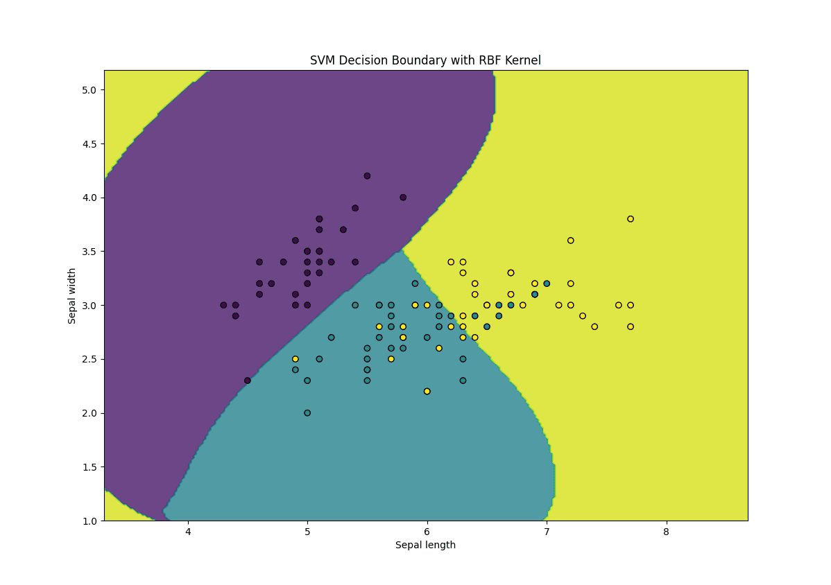
Here’s what’s going on in the above code:

• Kernel Selection: We use the RBF kernel (kernel=’rbf’) to handle non-linear data
• Gamma Parameter: The gamma parameter controls the influence of each training example, where a higher gamma value results in a more complex decision boundary
• C Parameter: The C parameter controls the trade-off between achieving a low training error and a low testing error

Kernel Principal Component Analysis (Kernel PCA)

Principal Component Analysis (PCA) is a dimensionality reduction technique that projects data onto a lower-dimensional space while preserving as much variance as possible. However, standard PCA is limited to linear transformations. Kernel PCA extends PCA by using kernel functions to perform non-linear dimensionality reduction.

Let’s implement Kernel PCA using scikit-learn and apply it to a non-linear dataset.

from sklearn.decomposition import KernelPCA from sklearn.datasets import make_moons   # Generate a non-linear dataset X, y = make_moons(n_samples=100, noise=0.1, random_state=42)   # Apply Kernel PCA with an RBF kernel kpca = KernelPCA(kernel='rbf', gamma=15, n_components=2) X_kpca = kpca.fit_transform(X)   # Plot the original data and the transformed data plt.figure(figsize=(12, 5))   plt.subplot(1, 2, 1) plt.scatter(X[:, 0], X[:, 1], c=y, edgecolors='k', marker='o') plt.title('Original Data')   plt.subplot(1, 2, 2) plt.scatter(X_kpca[:, 0], X_kpca[:, 1], c=y, edgecolors='k', marker='o') plt.title('Kernel PCA Transformed Data')   plt.show()

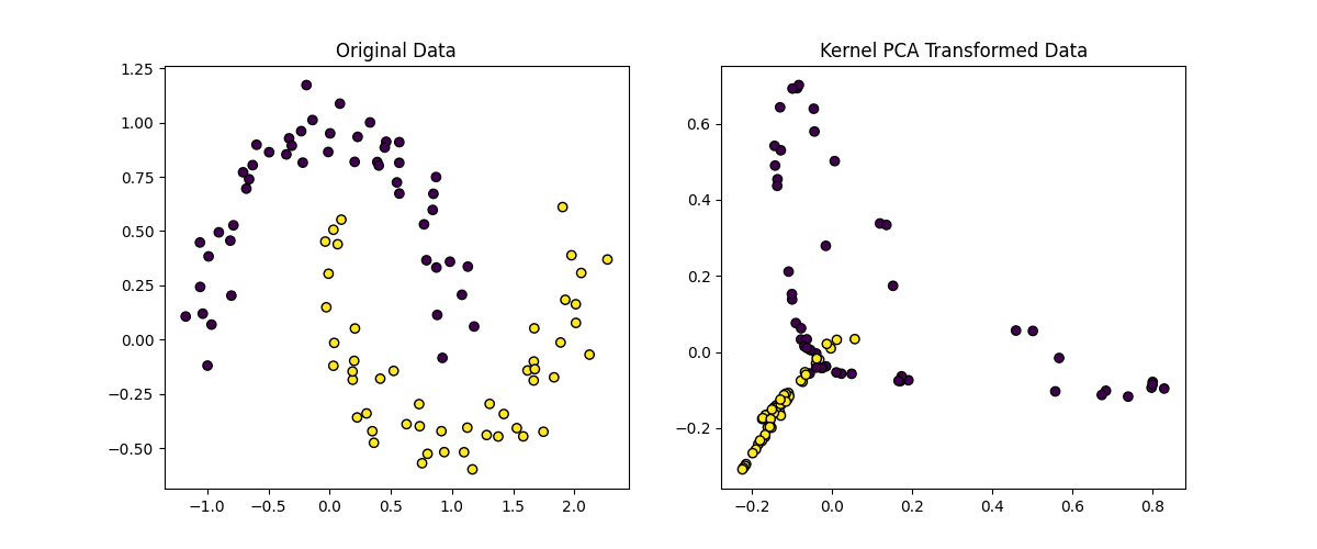
Here’s an explanation of the code above:

• Kernel Selection: We use the RBF kernel (kernel=’rbf’) to capture non-linear relationships in the data
• Gamma Parameter: The gamma parameter controls the influence of each data point, where a higher gamma value results in a more complex transformation
• Number of Components: We reduce the data to 2 dimensions (n_components=2) for visualization

Implementing the Kernel Trick from Scratch

A quick reminder: the kernel trick allows us to compute the dot product of two vectors in a high-dimensional space without explicitly mapping the vectors to that space. This is done using a kernel function, which directly computes the dot product in the transformed space.

Let’s implement the Radial Basis Function (RBF) kernel from scratch and use it to compute the kernel matrix for a dataset. The RBF kernel is defined as:

𝐾⁡(𝑥,𝑦)=exp⁡(−𝛾⁢‖𝑥–𝑦‖2)

Where:

• 𝑥 and 𝑦 are data points
• 𝛾 is a parameter that controls the influence of each data point, which we will refer to as gamma
• ‖𝑥–𝑦‖2 is the squared Euclidean distance between 𝑥 and 𝑦

Step 1: Define the RBF Kernel Function

Let’s start with the RBF kernel function.

import numpy as np   def rbf_kernel(x1, x2, gamma=1.0):     """     Compute the RBF kernel between two vectors x1 and x2.          Parameters:     - x1, x2: Input vectors.     - gamma: Kernel parameter.          Returns:     - Kernel value (scalar).     """     squared_distance = np.sum((x1 - x2) ** 2)     return np.exp(-gamma * squared_distance)

Step 2: Compute the Kernel Matrix

The kernel matrix (or Gram matrix) is a matrix where each element 𝐾𝑖⁢𝑗 is the kernel value between the 𝑖-th and 𝑗-th data points. Let’s compute the kernel matrix for a dataset.

def compute_kernel_matrix(X, kernel_function, gamma=1.0):     """     Compute the kernel matrix for a dataset X using a given kernel function.          Parameters:     - X: Input dataset (n_samples, n_features).     - kernel_function: Kernel function to use.     - gamma: Kernel parameter.          Returns:     - Kernel matrix (n_samples, n_samples).     """     n_samples = X.shape[0]     kernel_matrix = np.zeros((n_samples, n_samples))          for i in range(n_samples):         for j in range(n_samples):             kernel_matrix[i, j] = kernel_function(X[i], X[j], gamma)          return kernel_matrix

Step 3: Apply the Kernel Trick to a Simple Dataset

Let’s generate a simple 2D dataset and compute its kernel matrix using the RBF kernel.

# Generate a simple 2D dataset X = np.array([[1, 2], [2, 3], [3, 4], [4, 5]])   # Compute the kernel matrix using the RBF kernel gamma = 0.1 kernel_matrix = compute_kernel_matrix(X, rbf_kernel, gamma)   print("Kernel Matrix (RBF Kernel):") print(kernel_matrix)

The kernel matrix will look something like this:

Kernel Matrix (RBF Kernel): [[1.         0.81873075 0.44932896 0.16529889] [0.81873075 1.         0.81873075 0.44932896] [0.44932896 0.81873075 1.         0.81873075] [0.16529889 0.44932896 0.81873075 1.        ]]

Step 4: Use the Kernel Matrix in a Kernelized Algorithm

Now that we have the kernel matrix, we can use it in a kernelized algorithm, such as a kernel SVM. However, implementing a full kernel SVM from scratch is complex, so we’ll use the kernel matrix to demonstrate the concept.

For example, in a kernel SVM, the decision function for a new data point 𝑥 is computed as:

𝑓⁡(𝑥)=𝑛∑𝑖=1𝛼𝑖⁢𝑦𝑖⁢𝐾⁡(𝑥,𝑥𝑖)+𝑏

Where:

• 𝛼𝑖 are the Lagrange multipliers (learned during training).
• 𝑦𝑖 are the labels of the training data.
• 𝐾⁡(𝑥,𝑥𝑖) is the kernel value between 𝑥 and the 𝑖-th training point.
• 𝑏 is the bias term.

While we won’t implement the full SVM here, the kernel matrix is a crucial component of kernelized algorithms.

Here is a summary of the kernel trick implementation:

1. we implemented the RBF kernel function from scratch
2. we computed the kernel matrix for a dataset using the RBF kernel
3. the kernel matrix can be used in kernelized algorithms like kernel SVMs or kernel PCA

This implementation demonstrates the core idea of the kernel trick: working in a high-dimensional space without explicitly transforming the data. You can extend this approach to implement other kernel functions (e.g., polynomial kernel) or use the kernel matrix in custom kernelized algorithms.

Benefits of Kernel Trick vs. Explicit Transformation

So, why do we use the kernel trick instead of explicit transformation?

Explicit Transformation

Suppose we have a 2D dataset 𝑋 =[𝑥1,𝑥2] and we want to transform it into a higher-dimensional space using a polynomial transformation. For simplicity, let’s consider a quadratic transformation:

𝜙⁡(𝑥)=[𝑥1,𝑥2,𝑥21,𝑥22,𝑥1⁢𝑥2]

Here, 𝜙⁡(𝑥) maps the original 2D data into a 5D space. If we have 𝑛 data points, we would need to compute this transformation for each point, resulting in a 𝑛 ×5 matrix.

import numpy as np   # Original 2D data X = np.array([[1, 2], [2, 3], [3, 4]])   # Explicit transformation to 5D space def explicit_transformation(X):     x1 = X[:, 0]     x2 = X[:, 1]     return np.column_stack((x1, x2, x1**2, x2**2, x1 * x2))   # Apply the transformation X_transformed = explicit_transformation(X) print("Explicitly Transformed Data:") print(X_transformed)

And the output of the above code would be:

Explicitly Transformed Data: [[ 1  2  1  4  2] [ 2  3  4  9  6] [ 3  4  9 16 12]]

Here, we explicitly computed the new features in the 5D space. This works fine for small datasets and low-dimensional transformations, but it becomes problematic for:

• High-dimensional data: If the original data has many features, the transformed space can explode in size
• Complex transformations: Some transformations (e.g., RBF) map data into an infinite-dimensional space, which is impossible to compute explicitly.

Let’s now contrast this with the kernel trick.

Kernel Trick

The kernel trick avoids explicitly computing 𝜙⁡(𝑥) by directly computing the dot product 𝜙⁡(𝑥) ⋅𝜙⁡(𝑦) in the transformed space using a kernel function 𝐾⁡(𝑥,𝑦). For example, the RBF kernel implicitly maps data into an infinite-dimensional space, but we never compute 𝜙⁡(𝑥) directly.

# Kernel trick: Compute the dot product in the transformed space without explicit transformation def rbf_kernel(x1, x2, gamma=1.0):     squared_distance = np.sum((x1 - x2) ** 2)     return np.exp(-gamma * squared_distance)   # Compute the kernel matrix kernel_matrix = compute_kernel_matrix(X, rbf_kernel, gamma=1.0) print("Kernel Matrix (RBF Kernel):") print(kernel_matrix)

And the output:

Kernel Matrix (RBF Kernel): [[1.00000000e+00 1.35335283e-01 3.35462628e-04 1.52299797e-08] [1.35335283e-01 1.00000000e+00 1.35335283e-01 3.35462628e-04] [3.35462628e-04 1.35335283e-01 1.00000000e+00 1.35335283e-01] [1.52299797e-08 3.35462628e-04 1.35335283e-01 1.00000000e+00]]

Here, we never explicitly computed 𝜙⁡(𝑥). Instead, we used the kernel function to compute the dot product in the transformed space directly.

Method Comparison

Here’s why explicit transformation is problematic:

• Computational Cost: Explicitly transforming data into a high-dimensional space requires computing and storing the new features, which can be computationally expensive
• Infinite Dimensions: Some transformations (e.g., RBF) map data into an infinite-dimensional space, which is impossible to compute explicitly
• Memory Usage: Storing the transformed data can require a lot of memory, especially for large datasets

Explicit transformation TL;DR: Directly computes the transformed features 𝜙⁡(𝑥) in the higher-dimensional space. This is feasible for simple, low-dimensional transformations but becomes impractical for complex or high-dimensional transformations.

Conversely, the kernel trick is particularly useful when:

• The transformed feature space is very high-dimensional or infinite-dimensional
• You want to avoid the computational cost of explicitly transforming the data
• You are working with kernelized algorithms like SVMs, Kernel PCA, or Gaussian Processes

Kernel trick TL;DR: Avoids explicit transformation by computing the dot product 𝜙⁡(𝑥) ⋅𝜙⁡(𝑦) directly using a kernel function. This is efficient and works even for infinite-dimensional spaces. The kernel trick is a clever mathematical shortcut that allows us to work in high-dimensional spaces without the computational burden of explicit transformation.

Conclusion

Kernel methods are a powerful tool in machine learning, enabling us to handle non-linear data efficiently. In this tutorial, we explored the kernel trick, kernel SVMs, and Kernel PCA, and provided practical Python examples to help you get started with these techniques.

By mastering kernel methods, you can tackle a wide range of machine learning problems, from classification to dimensionality reduction, with greater flexibility and efficiency.