Moving Average Smoothing for Data Preparation and Time Series Forecasting in Python

 Moving average smoothing is a naive and effective technique in time series forecasting.

It can be used for data preparation, feature engineering, and even directly for making predictions.

In this tutorial, you will discover how to use moving average smoothing for time series forecasting with Python.

After completing this tutorial, you will know:

• How moving average smoothing works and some expectations of your data before you can use it.
• How to use moving average smoothing for data preparation and feature engineering.
• How to use moving average smoothing to make predictions.

Kick-start your project with my new book Time Series Forecasting With Python, including step-by-step tutorials and the Python source code files for all examples.

Let’s get started.

• Updated Apr/2019: Updated the link to dataset.
• Updated Aug/2019: Updated data loading to use new API.

Moving Average Smoothing for Data Preparation, Feature Engineering, and Time Series Forecasting with Python
Photo by Bureau of Land Management, some rights reserved.

Moving Average Smoothing

Smoothing is a technique applied to time series to remove the fine-grained variation between time steps.

The hope of smoothing is to remove noise and better expose the signal of the underlying causal processes. Moving averages are a simple and common type of smoothing used in time series analysis and time series forecasting.

Calculating a moving average involves creating a new series where the values are comprised of the average of raw observations in the original time series.

A moving average requires that you specify a window size called the window width. This defines the number of raw observations used to calculate the moving average value.

The “moving” part in the moving average refers to the fact that the window defined by the window width is slid along the time series to calculate the average values in the new series.

There are two main types of moving average that are used: Centered and Trailing Moving Average.

Centered Moving Average

The value at time (t) is calculated as the average of raw observations at, before, and after time (t).

For example, a center moving average with a window of 3 would be calculated as:

center_ma(t) = mean(obs(t-1), obs(t), obs(t+1))

This method requires knowledge of future values, and as such is used on time series analysis to better understand the dataset.

A center moving average can be used as a general method to remove trend and seasonal components from a time series, a method that we often cannot use when forecasting.

Trailing Moving Average

The value at time (t) is calculated as the average of the raw observations at and before the time (t).

For example, a trailing moving average with a window of 3 would be calculated as:

trail_ma(t) = mean(obs(t-2), obs(t-1), obs(t))

Trailing moving average only uses historical observations and is used on time series forecasting.

It is the type of moving average that we will focus on in this tutorial.

Data Expectations

Calculating a moving average of a time series makes some assumptions about your data.

It is assumed that both trend and seasonal components have been removed from your time series.

This means that your time series is stationary, or does not show obvious trends (long-term increasing or decreasing movement) or seasonality (consistent periodic structure).

There are many methods to remove trends and seasonality from a time series dataset when forecasting. Two good methods for each are to use the differencing method and to model the behavior and explicitly subtract it from the series.

Moving average values can be used in a number of ways when using machine learning algorithms on time series problems.

In this tutorial, we will look at how we can calculate trailing moving average values for use as data preparation, feature engineering, and for directly making predictions.

Before we dive into these examples, let’s look at the Daily Female Births dataset that we will use in each example.

Stop learning Time Series Forecasting the slow way!

Take my free 7-day email course and discover how to get started (with sample code).

Click to sign-up and also get a free PDF Ebook version of the course.

Daily Female Births Dataset

This dataset describes the number of daily female births in California in 1959.

The units are a count and there are 365 observations. The source of the dataset is credited to Newton (1988).

• Download the dataset.

Below is a sample of the first 5 rows of data, including the header row.

"Date","Births" "1959-01-01",35 "1959-01-02",32 "1959-01-03",30 "1959-01-04",31 "1959-01-05",44

Below is a plot of the entire dataset.

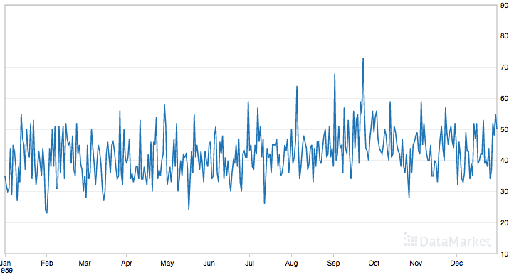
Daily Female Births Dataset

This dataset is a good example for exploring the moving average method as it does not show any clear trend or seasonality.

Load the Daily Female Births Dataset

Download the dataset and place it in the current working directory with the filename “daily-total-female-births.csv“.

The snippet below loads the dataset as a Series, displays the first 5 rows of the dataset, and graphs the whole series as a line plot.

from pandas import read_csv from matplotlib import pyplot series = read_csv('daily-total-female-births.csv', header=0, index_col=0) print(series.head()) series.plot() pyplot.show()

Running the example prints the first 5 rows as follows:

Date 1959-01-01 35 1959-01-02 32 1959-01-03 30 1959-01-04 31 1959-01-05 44

Below is the displayed line plot of the loaded data.

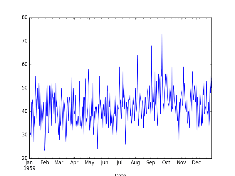
Daily Female Births Dataset Plot

Moving Average as Data Preparation

Moving average can be used as a data preparation technique to create a smoothed version of the original dataset.

Smoothing is useful as a data preparation technique as it can reduce the random variation in the observations and better expose the structure of the underlying causal processes.

The rolling() function on the Series Pandas object will automatically group observations into a window. You can specify the window size, and by default a trailing window is created. Once the window is created, we can take the mean value, and this is our transformed dataset.

New observations in the future can be just as easily transformed by keeping the raw values for the last few observations and updating a new average value.

To make this concrete, with a window size of 3, the transformed value at time (t) is calculated as the mean value for the previous 3 observations (t-2, t-1, t), as follows:

obs(t) = 1/3 * (t-2 + t-1 + t)

For the Daily Female Births dataset, the first moving average would be on January 3rd, as follows:

obs(t) = 1/3 * (t-2 + t-1 + t) obs(t) = 1/3 * (35 + 32 + 30) obs(t) = 32.333

Below is an example of transforming the Daily Female Births dataset into a moving average with a window size of 3 days, chosen arbitrarily.

from pandas import read_csv from matplotlib import pyplot series = read_csv('daily-total-female-births.csv', header=0, index_col=0) # Tail-rolling average transform rolling = series.rolling(window=3) rolling_mean = rolling.mean() print(rolling_mean.head(10)) # plot original and transformed dataset series.plot() rolling_mean.plot(color='red') pyplot.show()

Running the example prints the first 10 observations from the transformed dataset.

We can see that the first 2 observations will need to be discarded.

Date 1959-01-01          NaN 1959-01-02          NaN 1959-01-03    32.333333 1959-01-04    31.000000 1959-01-05    35.000000 1959-01-06    34.666667 1959-01-07    39.333333 1959-01-08    39.000000 1959-01-09    42.000000 1959-01-10    36.000000

The raw observations are plotted (blue) with the moving average transform overlaid (red).

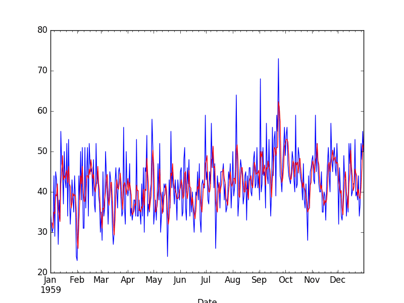
Moving Average Transform

To get a better idea of the effect of the transform, we can zoom in and plot the first 100 observations.

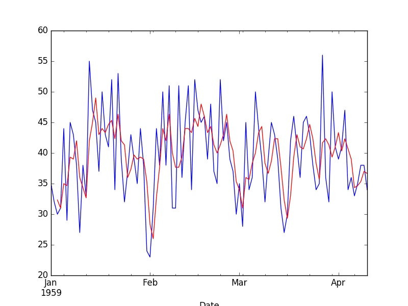
Zoomed Moving Average Transform

Here, you can clearly see the lag in the transformed dataset.

Next, let’s take a look at using the moving average as a feature engineering method.

Moving Average as Feature Engineering

The moving average can be used as a source of new information when modeling a time series forecast as a supervised learning problem.

In this case, the moving average is calculated and added as a new input feature used to predict the next time step.

First, a copy of the series must be shifted forward by one time step. This will represent the input to our prediction problem, or a lag=1 version of the series. This is a standard supervised learning view of the time series problem. For example:

X, y NaN, obs1 obs1, obs2 obs2, obs3

Next, a second copy of the series needs to be shifted forward by one, minus the window size. This is to ensure that the moving average summarizes the last few values and does not include the value to be predicted in the average, which would be an invalid framing of the problem as the input would contain knowledge of the future being predicted.

For example, with a window size of 3, we must shift the series forward by 2 time steps. This is because we want to include the previous two observations as well as the current observation in the moving average in order to predict the next value. We can then calculate the moving average from this shifted series.

Below is an example of how the first 5 moving average values are calculated. Remember, the dataset is shifted forward 2 time steps and as we move along the time series, it takes at least 3 time steps before we even have enough data to calculate a window=3 moving average.

Observations, Mean NaN NaN NaN, NaN NaN NaN, NaN, 35 NaN NaN, 35, 32 NaN 30, 32, 35 32

Below is an example of including the moving average of the previous 3 values as a new feature, as wellas a lag-1 input feature for the Daily Female Births dataset.

from pandas import read_csv from pandas import DataFrame from pandas import concat series = read_csv('daily-total-female-births.csv', header=0, index_col=0) df = DataFrame(series.values) width = 3 lag1 = df.shift(1) lag3 = df.shift(width - 1) window = lag3.rolling(window=width) means = window.mean() dataframe = concat([means, lag1, df], axis=1) dataframe.columns = ['mean', 't-1', 't+1'] print(dataframe.head(10))

Running the example creates the new dataset and prints the first 10 rows.

We can see that the first 3 rows cannot be used and must be discarded. The first row of the lag1 dataset cannot be used because there are no previous observations to predict the first observation, therefore a NaN value is used.

mean   t-1  t+1 0        NaN   NaN   35 1        NaN  35.0   32 2        NaN  32.0   30 3        NaN  30.0   31 4  32.333333  31.0   44 5  31.000000  44.0   29 6  35.000000  29.0   45 7  34.666667  45.0   43 8  39.333333  43.0   38 9  39.000000  38.0   27

The next section will look at how to use the moving average as a naive model to make predictions.

Moving Average as Prediction

The moving average value can also be used directly to make predictions.

It is a naive model and assumes that the trend and seasonality components of the time series have already been removed or adjusted for.

The moving average model for predictions can easily be used in a walk-forward manner. As new observations are made available (e.g. daily), the model can be updated and a prediction made for the next day.

We can implement this manually in Python. Below is an example of the moving average model used in a walk-forward manner.

from pandas import read_csv from numpy import mean from sklearn.metrics import mean_squared_error from matplotlib import pyplot series = read_csv('daily-total-female-births.csv', header=0, index_col=0) # prepare situation X = series.values window = 3 history = [X[i] for i in range(window)] test = [X[i] for i in range(window, len(X))] predictions = list() # walk forward over time steps in test for t in range(len(test)): length = len(history) yhat = mean([history[i] for i in range(length-window,length)]) obs = test[t] predictions.append(yhat) history.append(obs) print('predicted=%f, expected=%f' % (yhat, obs)) error = mean_squared_error(test, predictions) print('Test MSE: %.3f' % error) # plot pyplot.plot(test) pyplot.plot(predictions, color='red') pyplot.show() # zoom plot pyplot.plot(test[0:100]) pyplot.plot(predictions[0:100], color='red') pyplot.show()

Running the example prints the predicted and expected value each time step moving forward, starting from time step 4 (1959-01-04).

Finally, the mean squared error (MSE) is reported for all predictions made.

predicted=32.333333, expected=31.000000 predicted=31.000000, expected=44.000000 predicted=35.000000, expected=29.000000 predicted=34.666667, expected=45.000000 predicted=39.333333, expected=43.000000 ... predicted=38.333333, expected=52.000000 predicted=41.000000, expected=48.000000 predicted=45.666667, expected=55.000000 predicted=51.666667, expected=50.000000 Test MSE: 61.379

The example ends by plotting the expected test values (blue) compared to the predictions (red).

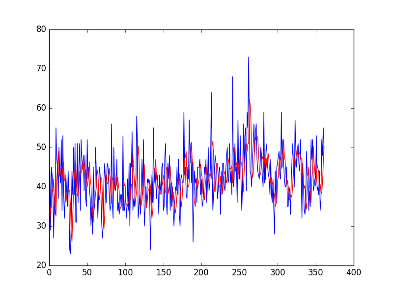
Moving Average Predictions

Again, zooming in on the first 100 predictions gives an idea of the skill of the 3-day moving average predictions.

Note the window width of 3 was chosen arbitrary and was not optimized.

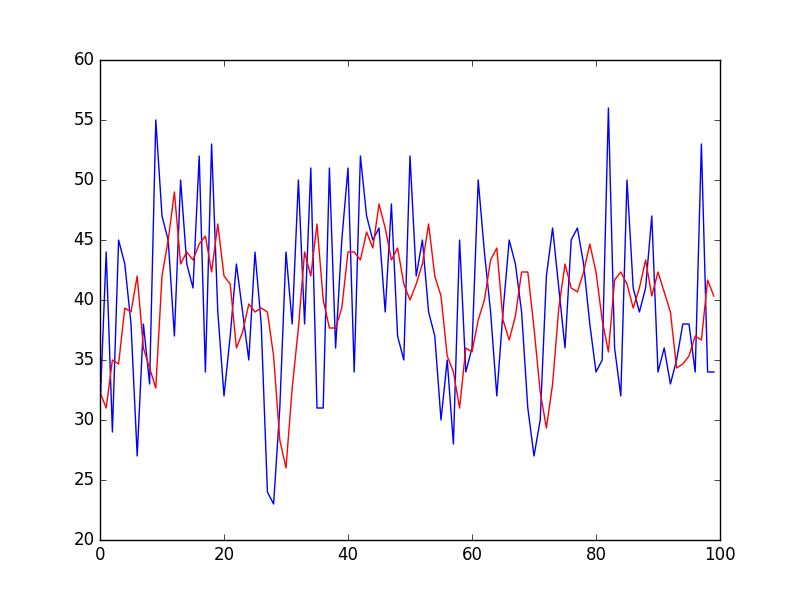
Zoomed Moving Average Predictions

Further Reading

This section lists some resources on smoothing moving averages for time series analysis and time series forecasting that you may find useful.

• Chapter 4, Smoothing Methods, Practical Time Series Forecasting with R: A Hands-On Guide.
• Section 1.5.4 Smoothing, Introductory Time Series with R.
• Section 2.4 Smoothing in the Time Series Context, Time Series Analysis and Its Applications: With R Examples.

Summary

In this tutorial, you discovered how to use moving average smoothing for time series forecasting with Python.

Specifically, you learned:

• How moving average smoothing works and the expectations of time series data before using it.
• How to use moving average smoothing for data preparation in Python.
• How to use moving average smoothing for feature engineering in Python.
• How to use moving average smoothing to make predictions in Python.

Do you have any questions about moving average smoothing, or about this tutorial?
Ask your questions in the comments below and I will do my best to answer.