How to Make Baseline Predictions for Time Series Forecasting with Python

 Establishing a baseline is essential on any time series forecasting problem.

A baseline in performance gives you an idea of how well all other models will actually perform on your problem.

In this tutorial, you will discover how to develop a persistence forecast that you can use to calculate a baseline level of performance on a time series dataset with Python.

After completing this tutorial, you will know:

• The importance of calculating a baseline of performance on time series forecast problems.
• How to develop a persistence model from scratch in Python.
• How to evaluate the forecast from a persistence model and use it to establish a baseline in performance.

Kick-start your project with my new book Time Series Forecasting With Python, including step-by-step tutorials and the Python source code files for all examples.

Let’s get started.

• Updated Apr/2019: Updated the link to dataset.

How to Make Baseline Predictions for Time Series Forecasting with Python
Photo by Bernard Spragg. NZ, some rights reserved.

Forecast Performance Baseline

A baseline in forecast performance provides a point of comparison.

It is a point of reference for all other modeling techniques on your problem. If a model achieves performance at or below the baseline, the technique should be fixed or abandoned.

The technique used to generate a forecast to calculate the baseline performance must be easy to implement and naive of problem-specific details.

Before you can establish a performance baseline on your forecast problem, you must develop a test harness. This is comprised of:

1. The dataset you intend to use to train and evaluate models.
2. The resampling technique you intend to use to estimate the performance of the technique (e.g. train/test split).
3. The performance measure you intend to use to evaluate forecasts (e.g. mean squared error).

Once prepared, you then need to select a naive technique that you can use to make a forecast and calculate the baseline performance.

The goal is to get a baseline performance on your time series forecast problem as quickly as possible so that you can get to work better understanding the dataset and developing more advanced models.

Three properties of a good technique for making a baseline forecast are:

• Simple: A method that requires little or no training or intelligence.
• Fast: A method that is fast to implement and computationally trivial to make a prediction.
• Repeatable: A method that is deterministic, meaning that it produces an expected output given the same input.

A common algorithm used in establishing a baseline performance is the persistence algorithm.

Stop learning Time Series Forecasting the slow way!

Take my free 7-day email course and discover how to get started (with sample code).

Click to sign-up and also get a free PDF Ebook version of the course.

Persistence Algorithm (the “naive” forecast)

The most common baseline method for supervised machine learning is the Zero Rule algorithm.

This algorithm predicts the majority class in the case of classification, or the average outcome in the case of regression. This could be used for time series, but does not respect the serial correlation structure in time series datasets.

The equivalent technique for use with time series dataset is the persistence algorithm.

The persistence algorithm uses the value at the previous time step (t-1) to predict the expected outcome at the next time step (t+1).

This satisfies the three above conditions for a baseline forecast.

To make this concrete, we will look at how to develop a persistence model and use it to establish a baseline performance for a simple univariate time series problem. First, let’s review the Shampoo Sales dataset.

Shampoo Sales Dataset

This dataset describes the monthly number of shampoo sales over a 3 year period.

The units are a sales count and there are 36 observations. The original dataset is credited to Makridakis, Wheelwright, and Hyndman (1998).

Below is a sample of the first 5 rows of data, including the header row.

"Month","Sales" "1-01",266.0 "1-02",145.9 "1-03",183.1 "1-04",119.3 "1-05",180.3

Below is a plot of the entire dataset where you can download the dataset and learn more about it.

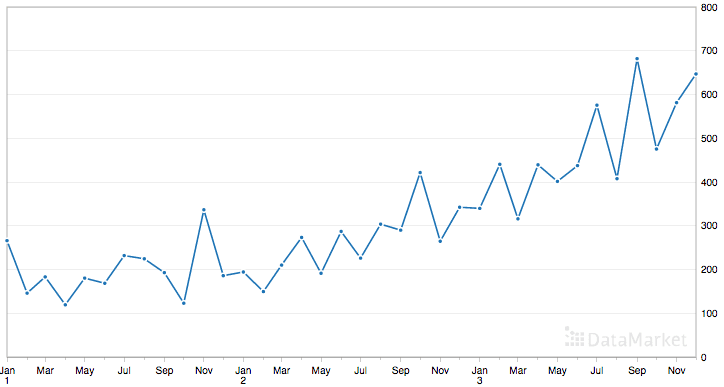
Shampoo Sales Dataset

The dataset shows an increasing trend, and possibly some seasonal component.

Download the dataset and place it in the current working directory with the filename “shampoo-sales.csv“.

• Download the dataset.

The following snippet of code will load the Shampoo Sales dataset and plot the time series.

from pandas import read_csv from pandas import datetime from matplotlib import pyplot   def parser(x): return datetime.strptime('190'+x, '%Y-%m')   series = read_csv('shampoo-sales.csv', header=0, parse_dates=[0], index_col=0, squeeze=True, date_parser=parser) series.plot() pyplot.show()

Running the example plots the time series, as follows:

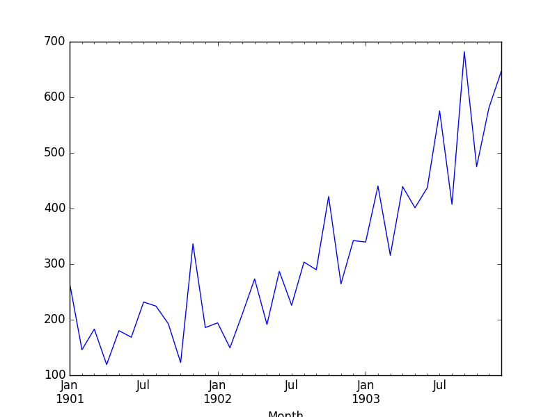
Shampoo Sales Dataset Plot

Persistence Algorithm

A persistence model can be implemented easily in Python.

We will break this section down into 4 steps:

1. Transform the univariate dataset into a supervised learning problem.
2. Establish the train and test datasets for the test harness.
3. Define the persistence model.
4. Make a forecast and establish a baseline performance.
5. Review the complete example and plot the output.

Let’s dive in.

Step 1: Define the Supervised Learning Problem

The first step is to load the dataset and create a lagged representation. That is, given the observation at t-1, predict the observation at t+1.

# Create lagged dataset values = DataFrame(series.values) dataframe = concat([values.shift(1), values], axis=1) dataframe.columns = ['t-1', 't+1'] print(dataframe.head(5))

This snippet creates the dataset and prints the first 5 rows of the new dataset.

We can see that the first row (index 0) will have to be discarded as there was no observation prior to the first observation to use to make the prediction.

From a supervised learning perspective, the t-1 column is the input variable, or X, and the t+1 column is the output variable, or y.

t-1    t+1 0    NaN  266.0 1  266.0  145.9 2  145.9  183.1 3  183.1  119.3 4  119.3  180.3

Step 2: Train and Test Sets

The next step is to separate the dataset into train and test sets.

We will keep the first 66% of the observations for “training” and the remaining 34% for evaluation. During the split, we are careful to exclude the first row of data with the NaN value.

No training is required in this case; it’s just habit. Each of the train and test sets are then split into the input and output variables.

# split into train and test sets X = dataframe.values train_size = int(len(X) * 0.66) train, test = X[1:train_size], X[train_size:] train_X, train_y = train[:,0], train[:,1] test_X, test_y = test[:,0], test[:,1]

Step 3: Persistence Algorithm

We can define our persistence model as a function that returns the value provided as input.

For example, if the t-1 value of 266.0 was provided, then this is returned as the prediction, whereas the actual real or expected value happens to be 145.9 (taken from the first usable row in our lagged dataset).

# persistence model def model_persistence(x): return x

Step 4: Make and Evaluate Forecast

Now we can evaluate this model on the test dataset.

We do this using the walk-forward validation method.

No model training or retraining is required, so in essence, we step through the test dataset time step by time step and get predictions.

Once predictions are made for each time step in the training dataset, they are compared to the expected values and a Mean Squared Error (MSE) score is calculated.

# walk-forward validation predictions = list() for x in test_X: yhat = model_persistence(x) predictions.append(yhat) test_score = mean_squared_error(test_y, predictions) print('Test MSE: %.3f' % test_score)

In this case, the error is more than 17,730 over the test dataset.

Test MSE: 17730.518

Step 5: Complete Example

Finally, a plot is made to show the training dataset and the diverging predictions from the expected values from the test dataset.

From the plot of the persistence model predictions, it is clear that the model is 1-step behind reality. There is a rising trend and month-to-month noise in the sales figures, which highlights the limitations of the persistence technique.

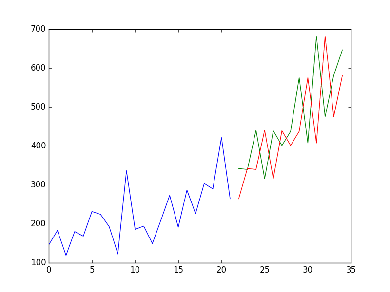
Shampoo Sales Persistence Model

The complete example is listed below.

from pandas import read_csv from pandas import datetime from pandas import DataFrame from pandas import concat from matplotlib import pyplot from sklearn.metrics import mean_squared_error   def parser(x): return datetime.strptime('190'+x, '%Y-%m')   series = read_csv('shampoo-sales.csv', header=0, parse_dates=[0], index_col=0, squeeze=True, date_parser=parser) # Create lagged dataset values = DataFrame(series.values) dataframe = concat([values.shift(1), values], axis=1) dataframe.columns = ['t-1', 't+1'] print(dataframe.head(5))   # split into train and test sets X = dataframe.values train_size = int(len(X) * 0.66) train, test = X[1:train_size], X[train_size:] train_X, train_y = train[:,0], train[:,1] test_X, test_y = test[:,0], test[:,1]   # persistence model def model_persistence(x): return x   # walk-forward validation predictions = list() for x in test_X: yhat = model_persistence(x) predictions.append(yhat) test_score = mean_squared_error(test_y, predictions) print('Test MSE: %.3f' % test_score)   # plot predictions and expected results pyplot.plot(train_y) pyplot.plot([None for i in train_y] + [x for x in test_y]) pyplot.plot([None for i in train_y] + [x for x in predictions]) pyplot.show()

We have seen an example of the persistence model developed from scratch for the Shampoo Sales problem.

The persistence algorithm is naive. It is often called the naive forecast.

It assumes nothing about the specifics of the time series problem to which it is applied. This is what makes it so easy to understand and so quick to implement and evaluate.

As a machine learning practitioner, it can also spark a large number of improvements.

Write them down.

This is useful because these ideas can become input features in a feature engineering effort or simple models that may be combined in an ensembling effort later.

Summary

In this tutorial, you discovered how to establish a baseline performance on time series forecast problems with Python.

Specifically, you learned:

• The importance of establishing a baseline and the persistence algorithm that you can use.
• How to implement the persistence algorithm in Python from scratch.
• How to evaluate the forecasts of the persistence algorithm and use them as a baseline.

Do you have any questions about baseline performance, or about this tutorial?
Ask your questions in the comments below and I will do my best to answer.