How to Use Features in LSTM Networks for Time Series Forecasting

 The Long Short-Term Memory (LSTM) network in Keras supports multiple input features.

This raises the question as to whether lag observations for a univariate time series can be used as features for an LSTM and whether or not this improves forecast performance.

In this tutorial, we will investigate the use of lag observations as features in LSTM models in Python.

After completing this tutorial, you will know:

• How to develop a test harness to systematically evaluate LSTM features for time series forecasting.
• The impact of using a varied number of lagged observations as input features for LSTM models.
• The impact of using a varied number of lagged observations and matching numbers of neurons for LSTM models.

  Tutorial Overview

  This tutorial is divided into 4 parts. They are:

  1. Shampoo Sales Dataset
  2. Experimental Test Harness
  3. Experiments with Timesteps
  4. Experiments with Timesteps and Neurons

  Environment

  This tutorial assumes you have a Python SciPy environment installed. You can use either Python 2 or 3 with this example.

  This tutorial assumes you have Keras v2.0 or higher installed with either the TensorFlow or Theano backend.

  This tutorial also assumes you have scikit-learn, Pandas, NumPy, and Matplotlib installed.

  Shampoo Sales Dataset

  This dataset describes the monthly number of sales of shampoo over a 3-year period.

  The units are a sales count and there are 36 observations. The original dataset is credited to Makridakis, Wheelwright, and Hyndman (1998).

  • Download the dataset.

  The example below loads and creates a plot of the loaded dataset.

  # load and plot dataset from pandas import read_csv from pandas import datetime from matplotlib import pyplot # load dataset def parser(x): return datetime.strptime('190'+x, '%Y-%m') series = read_csv('shampoo-sales.csv', header=0, parse_dates=[0], index_col=0, squeeze=True, date_parser=parser) # summarize first few rows print(series.head()) # line plot series.plot() pyplot.show()

  Running the example loads the dataset as a Pandas Series and prints the first 5 rows.

  Month 1901-01-01 266.0 1901-02-01 145.9 1901-03-01 183.1 1901-04-01 119.3 1901-05-01 180.3 Name: Sales, dtype: float64

  A line plot of the series is then created showing a clear increasing trend.

  

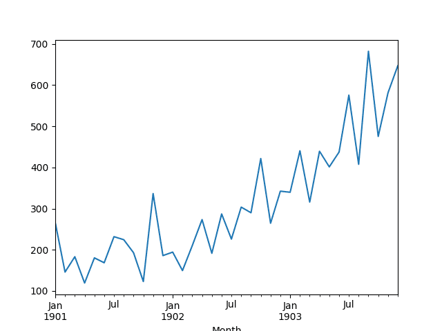
  Line Plot of Shampoo Sales Dataset

  Next, we will take a look at the LSTM configuration and test harness used in the experiment.

  Experimental Test Harness

  This section describes the test harness used in this tutorial.

  Data Split

  We will split the Shampoo Sales dataset into two parts: a training and a test set.

  The first two years of data will be taken for the training dataset and the remaining one year of data will be used for the test set.

  Models will be developed using the training dataset and will make predictions on the test dataset.

  The persistence forecast (naive forecast) on the test dataset achieves an error of 136.761 monthly shampoo sales. This provides a lower acceptable bound of performance on the test set.

  Model Evaluation

  A rolling-forecast scenario will be used, also called walk-forward model validation.

  Each time step of the test dataset will be walked one at a time. A model will be used to make a forecast for the time step, then the actual expected value from the test set will be taken and made available to the model for the forecast on the next time step.

  This mimics a real-world scenario where new Shampoo Sales observations would be available each month and used in the forecasting of the following month.

  This will be simulated by the structure of the train and test datasets.

  All forecasts on the test dataset will be collected and an error score calculated to summarize the skill of the model. The root mean squared error (RMSE) will be used as it punishes large errors and results in a score that is in the same units as the forecast data, namely monthly shampoo sales.

  Data Preparation

  Before we can fit an LSTM model to the dataset, we must transform the data.

  The following three data transforms are performed on the dataset prior to fitting a model and making a forecast.

  1. Transform the time series data so that it is stationary. Specifically, a lag=1 differencing to remove the increasing trend in the data.
  2. Transform the time series into a supervised learning problem. Specifically, the organization of data into input and output patterns where the observation at the previous time step is used as an input to forecast the observation at the current time step
  3. Transform the observations to have a specific scale. Specifically, to rescale the data to values between -1 and 1 to meet the default hyperbolic tangent activation function of the LSTM model.

  These transforms are inverted on forecasts to return them into their original scale before calculating and error score.

  LSTM Model

  We will use a base stateful LSTM model with 1 neuron fit for 500 epochs.

  A batch size of 1 is required as we will be using walk-forward validation and making one-step forecasts for each of the final 12 months of test data.

  A batch size of 1 means that the model will be fit using online training (as opposed to batch training or mini-batch training). As a result, it is expected that the model fit will have some variance.

  Ideally, more training epochs would be used (such as 1000 or 1500), but this was truncated to 500 to keep run times reasonable.

  The model will be fit using the efficient ADAM optimization algorithm and the mean squared error loss function.

  Experimental Runs

  Each experimental scenario will be run 10 times.

  The reason for this is that the random initial conditions for an LSTM network can result in very different results each time a given configuration is trained.

  Let’s dive into the experiments.

  Experiments with Features

  We will perform 5 experiments; each will use a different number of lag observations as features from 1 to 5.

  A representation with a 1 input feature would be the default representation when using a stateful LSTM. Using 2 to 5 features is contrived. The hope would be that the additional context from the lagged observations may improve performance of the predictive model.

  The univariate time series is converted to a supervised learning problem before training the model. The specified number of features defines the number of input variables (X) used to predict the next observation (y). As such, for each feature used in the representation, that many rows must be removed from the beginning of the dataset. This is because there are no prior observations to use as features for the first values in the dataset.

  The complete code listing for testing 1 input feature is provided below.

  The features parameter in the run() function is varied from 1 to 5 for each of the 5 experiments. In addition, the results are saved to file at the end of the experiment and this filename must also be changed for each different experimental run, e.g. experiment_features_1.csv, experiment_features_2.csv, etc.

  from pandas import DataFrame from pandas import Series from pandas import concat from pandas import read_csv from pandas import datetime from sklearn.metrics import mean_squared_error from sklearn.preprocessing import MinMaxScaler from keras.models import Sequential from keras.layers import Dense from keras.layers import LSTM from math import sqrt import matplotlib import numpy from numpy import concatenate   # date-time parsing function for loading the dataset def parser(x): return datetime.strptime('190'+x, '%Y-%m')   # frame a sequence as a supervised learning problem def timeseries_to_supervised(data, lag=1): df = DataFrame(data) columns = [df.shift(i) for i in range(1, lag+1)] columns.append(df) df = concat(columns, axis=1) return df   # create a differenced series def difference(dataset, interval=1): diff = list() for i in range(interval, len(dataset)): value = dataset[i] - dataset[i - interval] diff.append(value) return Series(diff)   # invert differenced value def inverse_difference(history, yhat, interval=1): return yhat + history[-interval]   # scale train and test data to [-1, 1] def scale(train, test): # fit scaler scaler = MinMaxScaler(feature_range=(-1, 1)) scaler = scaler.fit(train) # transform train train = train.reshape(train.shape[0], train.shape[1]) train_scaled = scaler.transform(train) # transform test test = test.reshape(test.shape[0], test.shape[1]) test_scaled = scaler.transform(test) return scaler, train_scaled, test_scaled   # inverse scaling for a forecasted value def invert_scale(scaler, X, yhat): new_row = [x for x in X] + [yhat] array = numpy.array(new_row) array = array.reshape(1, len(array)) inverted = scaler.inverse_transform(array) return inverted[0, -1]   # fit an LSTM network to training data def fit_lstm(train, batch_size, nb_epoch, neurons): X, y = train[:, 0:-1], train[:, -1] X = X.reshape(X.shape[0], 1, X.shape[1]) model = Sequential() model.add(LSTM(neurons, batch_input_shape=(batch_size, X.shape[1], X.shape[2]), stateful=True)) model.add(Dense(1)) model.compile(loss='mean_squared_error', optimizer='adam') for i in range(nb_epoch): model.fit(X, y, epochs=1, batch_size=batch_size, verbose=0, shuffle=False) model.reset_states() return model   # make a one-step forecast def forecast_lstm(model, batch_size, X): X = X.reshape(1, 1, len(X)) yhat = model.predict(X, batch_size=batch_size) return yhat[0,0]   # run a repeated experiment def experiment(repeats, series, features): # transform data to be stationary raw_values = series.values diff_values = difference(raw_values, 1) # transform data to be supervised learning supervised = timeseries_to_supervised(diff_values, features) supervised_values = supervised.values[features:,:] # split data into train and test-sets train, test = supervised_values[0:-12, :], supervised_values[-12:, :] # transform the scale of the data scaler, train_scaled, test_scaled = scale(train, test) # run experiment error_scores = list() for r in range(repeats): # fit the base model lstm_model = fit_lstm(train_scaled, 1, 500, 1) # forecast test dataset predictions = list() for i in range(len(test_scaled)): # predict X, y = test_scaled[i, 0:-1], test_scaled[i, -1] yhat = forecast_lstm(lstm_model, 1, X) # invert scaling yhat = invert_scale(scaler, X, yhat) # invert differencing yhat = inverse_difference(raw_values, yhat, len(test_scaled)+1-i) # store forecast predictions.append(yhat) # report performance rmse = sqrt(mean_squared_error(raw_values[-12:], predictions)) print('%d) Test RMSE: %.3f' % (r+1, rmse)) error_scores.append(rmse) return error_scores   # execute the experiment def run(): # load dataset series = read_csv('shampoo-sales.csv', header=0, parse_dates=[0], index_col=0, squeeze=True, date_parser=parser) # experiment repeats = 10 results = DataFrame() # run experiment features = 1 results['results'] = experiment(repeats, series, features) # summarize results print(results.describe()) # save results results.to_csv('experiment_features_1.csv', index=False)   # entry point run()

  Run the 5 different experiments for the 5 different numbers of features.

  You can run them in parallel if you have sufficient memory and CPU resources. GPU resources are not required for these experiments and runs should be complete in minutes to tens of minutes.

  After running the experiments, you should have 5 files containing the results, as follows:

  • experiment_features_1.csv
  • experiment_features_2.csv
  • experiment_features_3.csv
  • experiment_features_4.csv
  • experiment_features_5.csv

  We can write some code to load and summarize these results.

  Specifically, it is useful to review both descriptive statistics from each run and compare the results for each run using a box and whisker plot.

  Code to summarize the results is listed below.

  from pandas import DataFrame from pandas import read_csv from matplotlib import pyplot # load results into a dataframe filenames = ['experiment_features_1.csv', 'experiment_features_2.csv', 'experiment_features_3.csv','experiment_features_4.csv','experiment_features_5.csv'] results = DataFrame() for name in filenames: results[name[11:-4]] = read_csv(name, header=0) # describe all results print(results.describe()) # box and whisker plot results.boxplot() pyplot.show()

  Running the code first prints descriptive statistics for each set of results.

  Note: Your results may vary given the stochastic nature of the algorithm or evaluation procedure, or differences in numerical precision. Consider running the example a few times and compare the average outcome.

  We can see from the average performance alone that the default of using a single feature resulted in the best performance. This is also shown when reviewing the median test RMSE (50th percentile).

  features_1  features_2  features_3  features_4  features_5 count   10.000000   10.000000   10.000000   10.000000   10.000000 mean   104.588249  126.597800  118.268251  107.694178  116.414887 std     10.205840   18.639757   14.359983    8.683271   18.806281 min     89.046814   93.857991  103.900339   93.702085   98.245871 25%     97.850827  120.296634  107.664087  102.992045  105.660897 50%    103.713285  133.582095  116.123790  106.116922  112.950460 75%    111.441655  134.362198  121.794533  111.498255  117.926664 max    122.341580  149.807155  152.412861  123.006088  164.598542

  A box and whisker plot comparing the distributions of results is also created.

  The plot tells the same story as the descriptive statistics. The test RMSE seems to leap up with 2 features and trend upward as the number of features is increased.

  

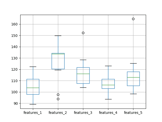
  Box and Whisker Plot of Test RMSE vs The Number of Input Features

  The expectation of decreased error with the increase of features was not observed, at least with the dataset and LSTM configuration used.

  This raises the question as to whether the capacity of the network is a limiting factor. We will look at this in the next section.

  Experiments with Features and Neurons

  The number of neurons (also called units) in the LSTM network defines its learning capacity.

  It is possible that in the previous experiments the use of one neuron limited the learning capacity of the network such that it was not capable of making effective use of the lagged observations as features.

  We can repeat the above experiments and increase the number of neurons in the LSTM with the increase in features and see if it results in an increase in performance.

  This can be achieved by changing the line in the experiment function from:

  lstm_model = fit_lstm(train_scaled, 1, 500, 1, features)

  to

  lstm_model = fit_lstm(train_scaled, 1, 500, features, features)

  In addition, we can keep the results written to file separate from the results from the first experiment by adding a “_neurons” suffix to the filenames, for example, changing:

  results.to_csv('experiment_features_1.csv', index=False)

  to

  results.to_csv('experiment_features_1_neurons.csv', index=False)

  Repeat the same 5 experiments with these changes.

  After running these experiments, you should have 5 result files.

  • experiment_features_1_neurons.csv
  • experiment_features_2_neurons.csv
  • experiment_features_3_neurons.csv
  • experiment_features_4_neurons.csv
  • experiment_features_5_neurons.csv

  As in the previous experiment, we can load the results, calculate descriptive statistics, and create a box and whisker plot. The complete code listing is below.

  from pandas import DataFrame from pandas import read_csv from matplotlib import pyplot # load results into a dataframe filenames = ['experiment_features_1_neurons.csv', 'experiment_features_2_neurons.csv', 'experiment_features_3_neurons.csv','experiment_features_4_neurons.csv','experiment_features_5_neurons.csv'] results = DataFrame() for name in filenames: results[name[11:-12]] = read_csv(name, header=0) # describe all results print(results.describe()) # box and whisker plot results.boxplot() pyplot.show()

  Running the code first prints descriptive statistics from each of the 5 experiments.

  Note: Your results may vary given the stochastic nature of the algorithm or evaluation procedure, or differences in numerical precision. Consider running the example a few times and compare the average outcome.

  The results tell a different story to the first set of experiments with a one neuron LSTM. The average test RMSE appears lowest when the number of neurons and the number of features is set to one, then error increases as neurons and features are increased.

  features_1  features_2  features_3  features_4  features_5 count   10.000000   10.000000   10.000000   10.000000   10.000000 mean   106.219189  138.411111  127.687128  154.281694  175.951500 std     16.100488   29.700981   21.411766   30.526294   44.839217 min     91.073598   92.641030  103.503546   94.063639  117.017109 25%     97.263723  125.748973  108.972440  134.805621  142.146601 50%     99.036766  133.639168  128.627349  162.295657  182.406707 75%    110.625302  146.896608  134.012859  176.969980  197.913894 max    146.638148  206.760081  170.899267  188.911768  250.685187

  A box and whisker plot is created to compare the distributions.

  The trend in spread and median performance almost shows a linear increase in test RMSE as the number of neurons and input features is increased.

  The linear trend may suggest that the increase network capacity is not given sufficient time to fit the data. Perhaps an increase in the number of epochs would be required as well.

  

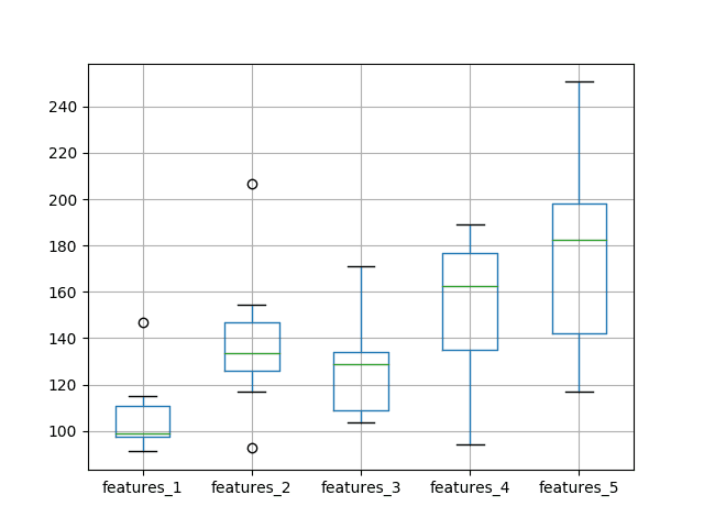
  Box and Whisker Plot of Test RMSE vs The Number of Neurons and Input Features

  Experiments with Features and Neurons More Epochs

  In this section, we repeat the above experiment to increase the number of neurons with the number of features but double the number of training epochs from 500 to 1000.

  This can be achieved by changing the line in the experiment function from:

  lstm_model = fit_lstm(train_scaled, 1, 500, features, features)

  to

  lstm_model = fit_lstm(train_scaled, 1, 1000, features, features)

  In addition, we can keep the results written to file separate from the results from the previous experiment by adding a “1000” suffix to the filenames, for example, changing:

  results.to_csv('experiment_features_1_neurons.csv', index=False)

  to

  results.to_csv('experiment_features_1_neurons1000.csv', index=False)

  Repeat the same 5 experiments with these changes.

  After running these experiments, you should have 5 result files.

  • experiment_features_1_neurons1000.csv
  • experiment_features_2_neurons1000.csv
  • experiment_features_3_neurons1000.csv
  • experiment_features_4_neurons1000.csv
  • experiment_features_5_neurons1000.csv

  As in the previous experiment, we can load the results, calculate descriptive statistics, and create a box and whisker plot. The complete code listing is below.

  from pandas import DataFrame from pandas import read_csv from matplotlib import pyplot # load results into a dataframe filenames = ['experiment_features_1_neurons1000.csv', 'experiment_features_2_neurons1000.csv', 'experiment_features_3_neurons1000.csv','experiment_features_4_neurons1000.csv','experiment_features_5_neurons1000.csv'] results = DataFrame() for name in filenames: results[name[11:-16]] = read_csv(name, header=0) # describe all results print(results.describe()) # box and whisker plot results.boxplot() pyplot.show()

  Running the code first prints descriptive statistics from each of the 5 experiments.

  Note: Your results may vary given the stochastic nature of the algorithm or evaluation procedure, or differences in numerical precision. Consider running the example a few times and compare the average outcome.

  The results tell a very similar story to the previous experiment with half the number of training epochs. On average, a model with 1 input feature and 1 neuron outperformed the other configurations.

  features_1  features_2  features_3  features_4  features_5 count   10.000000   10.000000   10.000000   10.000000   10.000000 mean   109.262674  158.295172  120.340623  149.741882  201.992209 std     13.850525   32.288109   45.219564   53.121113   82.986691 min     95.927393  111.936394   83.983325  111.017837   78.040385 25%     98.754253  130.875314   95.198556  122.287208  148.840499 50%    103.990988  167.915523  110.256517  129.552084  188.498836 75%    116.055435  180.679252  122.158321  154.283676  234.519359 max    133.270446  204.260072  242.186747  288.907803  335.595974

  A box and whisker plot was also created to compare the distributions. In the plot, we see the same trend as was clear in the descriptive statistics.

  At least on this problem and with the chosen LSTM configuration, we do not see any clear benefit in increasing the number of input features.

  

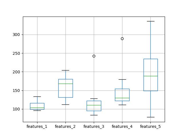
  Box and Whisker Plot of Test RMSE vs The Number of Neurons and Input Features and 1000 Epochs

  Extensions

  This section lists some areas for further investigation that you may consider exploring.

  • Diagnostic Run Plots. It may be helpful to review plots of train and test RMSE over epochs for multiple runs for a given experiment. This might help tease out whether overfitting or underfitting is taking place, and in turn, methods to address it.
  • Increase Repeats. Using 10 repeats results in a relatively small population of test RMSE results. It is possible that increasing repeats to 30 or 100 (or even higher) may result in a more stable outcome.

  Did you explore any of these extensions?
  Share your findings in the comments below; I’d love to hear what you found.

  Summary

  In this tutorial, you discovered how to investigate using lagged observations as input features in an LSTM network.

  Specifically, you learned:

  • How to develop a robust test harness for experimenting with input representation with LSTMs.
  • How to use lagged observations as input features for time series forecasting with LSTMs.
  • How to increase the learning capacity of the network with the increase of input features.

  You discovered that the expectation that “the use of lagged observations as input features improves model skill” did not decrease the test RMSE on the chosen problem and LSTM configuration.

  Do you have any questions?
  Ask your questions in the comments below and I will do my best to answer them.