Stateful and Stateless LSTM for Time Series Forecasting with Python

 The Keras Python deep learning library supports both stateful and stateless Long Short-Term Memory (LSTM) networks.

When using stateful LSTM networks, we have fine-grained control over when the internal state of the LSTM network is reset. Therefore, it is important to understand different ways of managing this internal state when fitting and making predictions with LSTM networks affect the skill of the network.

In this tutorial, you will explore the performance of stateful and stateless LSTM networks in Keras for time series forecasting.

After completing this tutorial, you will know:

• How to compare and contrast stateful and stateless LSTM networks for time series forecasts.
• How the batch size in stateless LSTMs relate to stateful LSTM networks.
• How to evaluate and compare different state resetting regimes for stateful LSTM networks

  Tutorial Overview

  This tutorial is broken down into 7 parts. They are:

  1. Shampoo Sales Dataset
  2. Experimental Test Harness
  3. A vs A Test
  4. Stateful vs Stateless
  5. Stateless With Large Batch vs Stateless
  6. Stateful Resetting vs Stateless
  7. Review of Findings

  Environment

  This tutorial assumes you have a Python SciPy environment installed. You can use either Python 2 or 3 with this example.

  This tutorial assumes you have Keras v2.0 or higher installed with either the TensorFlow or Theano backend.

  This tutorial also assumes you have scikit-learn, Pandas, NumPy, and Matplotlib installed.

  Shampoo Sales Dataset

  This dataset describes the monthly number of sales of shampoo over a 3-year period.

  The units are a sales count and there are 36 observations. The original dataset is credited to Makridakis, Wheelwright, and Hyndman (1998).

  • Download the dataset.

  The example below loads and creates a plot of the loaded dataset.

  # load and plot dataset from pandas import read_csv from pandas import datetime from matplotlib import pyplot # load dataset def parser(x): return datetime.strptime('190'+x, '%Y-%m') series = read_csv('shampoo-sales.csv', header=0, parse_dates=[0], index_col=0, squeeze=True, date_parser=parser) # summarize first few rows print(series.head()) # line plot series.plot() pyplot.show()

  Running the example loads the dataset as a Pandas Series and prints the first 5 rows.

  Month 1901-01-01 266.0 1901-02-01 145.9 1901-03-01 183.1 1901-04-01 119.3 1901-05-01 180.3 Name: Sales, dtype: float64

  A line plot of the series is then created showing a clear increasing trend.

  

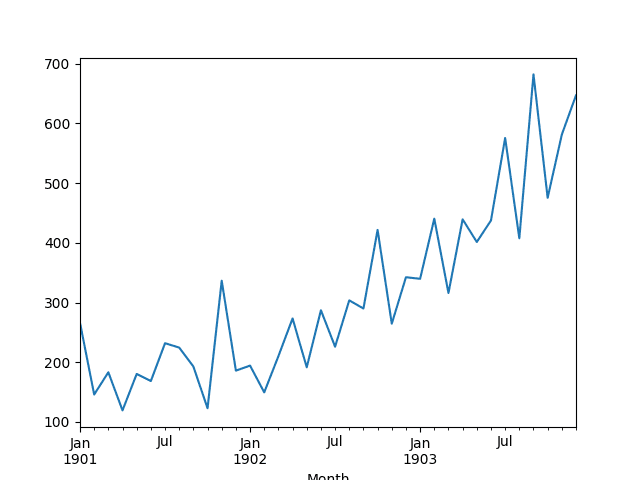
  Line Plot of Shampoo Sales Dataset

  Next, we will take a look at the LSTM configuration and test harness used in the experiment.

  Experimental Test Harness

  This section describes the test harness used in this tutorial.

  Data Split

  We will split the Shampoo Sales dataset into two parts: a training and a test set.

  The first two years of data will be taken for the training dataset and the remaining one year of data will be used for the test set.

  Models will be developed using the training dataset and will make predictions on the test dataset.

  The persistence forecast (naive forecast) on the test dataset achieves an error of 136.761 monthly shampoo sales. This provides a lower acceptable bound of performance on the test set.

  Model Evaluation

  A rolling-forecast scenario will be used, also called walk-forward model validation.

  Each time step of the test dataset will be walked one at a time. A model will be used to make a forecast for the time step, then the actual expected value from the test set will be taken and made available to the model for the forecast on the next time step.

  This mimics a real-world scenario where new Shampoo Sales observations would be available each month and used in the forecasting of the following month.

  This will be simulated by the structure of the train and test datasets.

  All forecasts on the test dataset will be collected and an error score calculated to summarize the skill of the model. The root mean squared error (RMSE) will be used as it punishes large errors and results in a score that is in the same units as the forecast data, namely monthly shampoo sales.

  Data Preparation

  Before we can fit an LSTM model to the dataset, we must transform the data.

  The following three data transforms are performed on the dataset prior to fitting a model and making a forecast.

  1. Transform the time series data so that it is stationary. Specifically, a lag=1 differencing to remove the increasing trend in the data.
  2. Transform the time series into a supervised learning problem. Specifically, the organization of data into input and output patterns where the observation at the previous time step is used as an input to forecast the observation at the current time step
  3. Transform the observations to have a specific scale. Specifically, to rescale the data to values between -1 and 1 to meet the default hyperbolic tangent activation function of the LSTM model.

  These transforms are inverted on forecasts to return them into their original scale before calculating and error score.

  LSTM Model

  We will use a base stateful LSTM model with 1 neuron fit for 1000 epochs.

  A batch size of 1 is required as we will be using walk-forward validation and making one-step forecasts for each of the final 12 months of test data.

  A batch size of 1 means that the model will be fit using online training (as opposed to batch training or mini-batch training). As a result, it is expected that the model fit will have some variance.

  Ideally, more training epochs would be used (such as 1500), but this was truncated to 1000 to keep run times reasonable.

  The model will be fit using the efficient ADAM optimization algorithm and the mean squared error loss function.

  Experimental Runs

  Each experimental scenario will be run 10 times.

  The reason for this is that the random initial conditions for an LSTM network can result in very different results each time a given configuration is trained.

  Let’s dive into the experiments.

  A vs A Test

  A good first experiment is to evaluate how noisy or reliable our test harness may be.

  This can be evaluated by running the same experiment twice and comparing the results. This is often called an A vs A test in the world of A/B testing, and I find this name useful. The idea is to flush out any obvious faults with the experiment and get a handle on the expected variance in the mean value.

  We will run an experiment with a stateful LSTM on the network twice.

  The complete code listing is provided below.

  This code also provides the basis for all experiments in this tutorial. Rather than re-listing it for each variation in subsequent sections, I will only list the functions that have been changed.

  from pandas import DataFrame from pandas import Series from pandas import concat from pandas import read_csv from pandas import datetime from sklearn.metrics import mean_squared_error from sklearn.preprocessing import MinMaxScaler from keras.models import Sequential from keras.layers import Dense from keras.layers import LSTM from math import sqrt import matplotlib import numpy from numpy import concatenate   # date-time parsing function for loading the dataset def parser(x): return datetime.strptime('190'+x, '%Y-%m')   # frame a sequence as a supervised learning problem def timeseries_to_supervised(data, lag=1): df = DataFrame(data) columns = [df.shift(i) for i in range(1, lag+1)] columns.append(df) df = concat(columns, axis=1) return df   # create a differenced series def difference(dataset, interval=1): diff = list() for i in range(interval, len(dataset)): value = dataset[i] - dataset[i - interval] diff.append(value) return Series(diff)   # invert differenced value def inverse_difference(history, yhat, interval=1): return yhat + history[-interval]   # scale train and test data to [-1, 1] def scale(train, test): # fit scaler scaler = MinMaxScaler(feature_range=(-1, 1)) scaler = scaler.fit(train) # transform train train = train.reshape(train.shape[0], train.shape[1]) train_scaled = scaler.transform(train) # transform test test = test.reshape(test.shape[0], test.shape[1]) test_scaled = scaler.transform(test) return scaler, train_scaled, test_scaled   # inverse scaling for a forecasted value def invert_scale(scaler, X, yhat): new_row = [x for x in X] + [yhat] array = numpy.array(new_row) array = array.reshape(1, len(array)) inverted = scaler.inverse_transform(array) return inverted[0, -1]   # fit an LSTM network to training data def fit_lstm(train, batch_size, nb_epoch, neurons): X, y = train[:, 0:-1], train[:, -1] X = X.reshape(X.shape[0], 1, X.shape[1]) model = Sequential() model.add(LSTM(neurons, batch_input_shape=(batch_size, X.shape[1], X.shape[2]), stateful=True)) model.add(Dense(1)) model.compile(loss='mean_squared_error', optimizer='adam') for i in range(nb_epoch): model.fit(X, y, epochs=1, batch_size=batch_size, verbose=0, shuffle=False) model.reset_states() return model   # make a one-step forecast def forecast_lstm(model, batch_size, X): X = X.reshape(1, 1, len(X)) yhat = model.predict(X, batch_size=batch_size) return yhat[0,0]   # run a repeated experiment def experiment(repeats, series): # transform data to be stationary raw_values = series.values diff_values = difference(raw_values, 1) # transform data to be supervised learning supervised = timeseries_to_supervised(diff_values, 1) supervised_values = supervised.values[1:,:] # split data into train and test-sets train, test = supervised_values[0:-12, :], supervised_values[-12:, :] # transform the scale of the data scaler, train_scaled, test_scaled = scale(train, test) # run experiment error_scores = list() for r in range(repeats): # fit the base model lstm_model = fit_lstm(train_scaled, 1, 1000, 1) # forecast test dataset predictions = list() for i in range(len(test_scaled)): # predict X, y = test_scaled[i, 0:-1], test_scaled[i, -1] yhat = forecast_lstm(lstm_model, 1, X) # invert scaling yhat = invert_scale(scaler, X, yhat) # invert differencing yhat = inverse_difference(raw_values, yhat, len(test_scaled)+1-i) # store forecast predictions.append(yhat) # report performance rmse = sqrt(mean_squared_error(raw_values[-12:], predictions)) print('%d) Test RMSE: %.3f' % (r+1, rmse)) error_scores.append(rmse) return error_scores   # execute the experiment def run(): # load dataset series = read_csv('shampoo-sales.csv', header=0, parse_dates=[0], index_col=0, squeeze=True, date_parser=parser) # experiment repeats = 10 results = DataFrame() # run experiment results['results'] = experiment(repeats, series) # summarize results print(results.describe()) # save results results.to_csv('experiment_stateful.csv', index=False)   # entry point run()

  Running the experiment saves the results to a file named “experiment_stateful.csv“.

  Run the experiment a second time and change the filename written by the experiment to “experiment_stateful2.csv” as to not overwrite the results from the first run.

  You should now have two sets of results in the current working directory in the files:

  • experiment_stateful.csv
  • experiment_stateful2.csv

  We can now load and compare these two files. The script to do this is listed below.

  from pandas import DataFrame from pandas import read_csv from matplotlib import pyplot # load results into a dataframe filenames = ['experiment_stateful.csv', 'experiment_stateful2.csv'] results = DataFrame() for name in filenames: results[name[11:-4]] = read_csv(name, header=0) # describe all results print(results.describe()) # box and whisker plot results.boxplot() pyplot.show()

  This script loads the result files and first calculates descriptive statistics for each run.

  Note: Your results may vary given the stochastic nature of the algorithm or evaluation procedure, or differences in numerical precision. Consider running the example a few times and compare the average outcome.

  We can see that the mean results and standard deviation are relatively close values (around 103-106 and 7-10 respectively). This is a good sign, but not perfect. It is expected that increasing the number of repeats of the experiment from 10 to 30, 100, or even 1000 would produce near identical summary statistics.

  stateful   stateful2 count   10.000000   10.000000 mean   103.142903  106.594624 std      7.109461   10.687509 min     94.052380   91.570179 25%     96.765985  101.015403 50%    104.376252  102.425406 75%    107.753516  115.024920 max    114.958430  125.088436

  The comparison also creates a box and whisker plot to compare the two distributions.

  The plot shows the 25th, 50th (median), and 75th percentile of 10 test RMSE results from each experiment. The box shows the middle 50% of the data and the green line shows the median.

  The plot shows that although the descriptive statistics are reasonably close, the distributions do show some differences.

  Nevertheless, the distributions do overlap and comparing means and standard deviations of different experimental setups is reasonable as long as we don’t quibble over modest differences in mean.

  

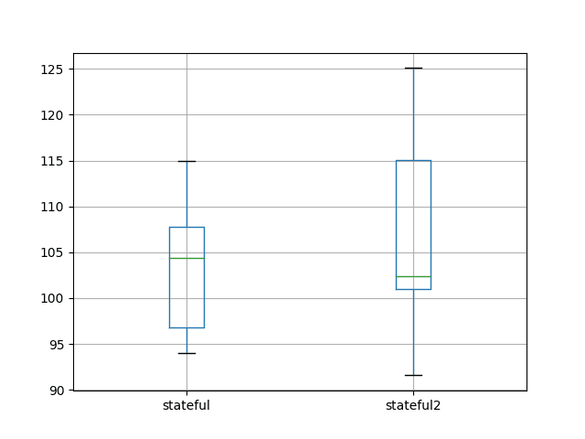
  Box and Whisker Plot of A vs A Experimental Results

  A good follow-up to this analysis is to review the standard error of the distribution with different sample sizes. This would involve first creating a larger pool of experimental runs from which to draw (100 or 1000), and would give a good idea of a robust number of repeats and an expected error on the mean when comparing results.

  Stateful vs Stateless LSTMs

  A good first experiment is to explore whether maintaining state in the LSTM adds value over not maintaining state.

  In this section, we will contrast:

  1. A Stateful LSTM (first result from the previous section).
  2. A Stateless LSTM with the same configuration.
  3. A Stateless LSTM with shuffling during training.

  The benefit of LSTM networks is their ability to maintain state and learn a sequence.

  • Expectation 1: The expectation is that the stateful LSTM will outperform the stateless LSTM.

  Shuffling of input patterns each batch or epoch is often performed to improve the generalizability of an MLP network during training. A stateless LSTM does not shuffle input patterns during training because the network aims to learn the sequence of patterns. We will test a stateless LSTM with and without shuffling.

  • Expectation 2: The expectation is that the stateless LSTM without shuffling will outperform the stateless LSTM with shuffling.

  The code changes to the stateful LSTM example above to make it stateless involve setting stateful=False in the LSTM layer and the use of automated training epoch training rather than manual. The results are written to a new file named “experiment_stateless.csv“. The updated fit_lstm() function is listed below.

  # fit an LSTM network to training data def fit_lstm(train, batch_size, nb_epoch, neurons): X, y = train[:, 0:-1], train[:, -1] X = X.reshape(X.shape[0], 1, X.shape[1]) model = Sequential() model.add(LSTM(neurons, batch_input_shape=(batch_size, X.shape[1], X.shape[2]), stateful=False)) model.add(Dense(1)) model.compile(loss='mean_squared_error', optimizer='adam') model.fit(X, y, epochs=nb_epoch, batch_size=batch_size, verbose=0, shuffle=False) return model

  The stateless with shuffling experiment involves setting the shuffle argument to True when calling fit in the fit_lstm() function. The results from this experiment are written to the file “experiment_stateless_shuffle.csv“.

  The complete updated fit_lstm() function is listed below.

  # fit an LSTM network to training data def fit_lstm(train, batch_size, nb_epoch, neurons): X, y = train[:, 0:-1], train[:, -1] X = X.reshape(X.shape[0], 1, X.shape[1]) model = Sequential() model.add(LSTM(neurons, batch_input_shape=(batch_size, X.shape[1], X.shape[2]), stateful=False)) model.add(Dense(1)) model.compile(loss='mean_squared_error', optimizer='adam') model.fit(X, y, epochs=nb_epoch, batch_size=batch_size, verbose=0, shuffle=True) return model

  After running the experiments, you should have three result files for comparison:

  • experiment_stateful.csv
  • experiment_stateless.csv
  • experiment_stateless_shuffle.csv

  We can now load and compare these results. The complete example for comparing the results is listed below.

  from pandas import DataFrame from pandas import read_csv from matplotlib import pyplot # load results into a dataframe filenames = ['experiment_stateful.csv', 'experiment_stateless.csv', 'experiment_stateless_shuffle.csv'] results = DataFrame() for name in filenames: results[name[11:-4]] = read_csv(name, header=0) # describe all results print(results.describe()) # box and whisker plot results.boxplot() pyplot.show()

  Running the example first calculates and prints descriptive statistics for each of the experiments.

  Note: Your results may vary given the stochastic nature of the algorithm or evaluation procedure, or differences in numerical precision. Consider running the example a few times and compare the average outcome.

  The average results suggest that the stateless LSTM configurations may outperform the stateful configuration. If robust, this finding is quite surprising as it does not meet the expectation of the addition of state improving performance.

  The shuffling of training samples does not appear to make a large difference to the stateless LSTM. If the result is robust, the expectation of shuffled training order on the stateless LSTM does appear to offer some benefit.

  Together, these findings may further suggest that the chosen LSTM configuration is focused more on learning input-output pairs rather than dependencies within the sequence.

  From these limited results alone, one would consider exploring stateless LSTMs on this problem.

  stateful   stateless  stateless_shuffle count   10.000000   10.000000          10.000000 mean   103.142903   95.661773          96.206332 std      7.109461    1.924133           2.138610 min     94.052380   94.097259          93.678941 25%     96.765985   94.290720          94.548002 50%    104.376252   95.098050          95.804411 75%    107.753516   96.092609          97.076086 max    114.958430  100.334725          99.870445

  A box and whisker plot is also created to compare the distributions.

  The spread of the data appears much larger with the stateful configuration compared to the stateless cases. This is also present in the descriptive statistics when we look at the standard deviation scores.

  This suggests that the stateless configurations may be more stable.

  

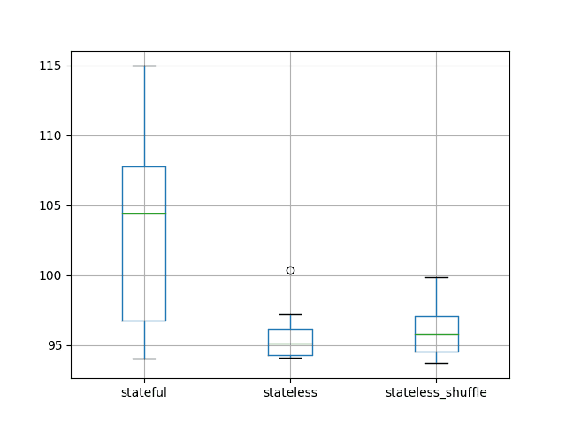
  Box and Whisker Plot of Test RMSE of Stateful vs Stateless LSTM Results

  Stateless with Large Batch vs Stateless

  A key to understanding the difference between stateful and stateless LSTMs is “when internal state is reset”.

  • Stateless: In the stateless LSTM configuration, internal state is reset after each training batch or each batch when making predictions.
  • Stateful: In the stateful LSTM configuration, internal state is only reset when the reset_state() function is called.

  If this is the only difference, then it may be possible to simulate a stateful LSTM with a stateless LSTM using a large batch size.

  • Expectation 3: Stateless and stateful LSTMs should produce near identical results when using the same batch size.

  We can do this with the Shampoo Sales dataset by truncating the training data to only 12 months and leaving the test data as 12 months. This would allow a stateless LSTM to use a batch size of 12. If training and testing were performed in a one-shot manner (one function call), then it is possible that internal state of the “stateless” LSTM would not be reset and both configurations would produce equivalent results.

  We will use the stateful results from the first experiment as a starting point. The forecast_lstm() function is modified to forecast one year of observations in a single step. The experiment() function is modified to truncate the training dataset to 12 months of data, to use a batch size of 12, and to process the batched predictions returned from the forecast_lstm() function. These updated functions are listed below. Results are written to the file “experiment_stateful_batch12.csv“.

  # make a one-step forecast def forecast_lstm(model, batch_size, X): X = X.reshape(1, 1, len(X)) yhat = model.predict(X, batch_size=batch_size) return yhat[0,0]   # run a repeated experiment def experiment(repeats, series): # transform data to be stationary raw_values = series.values diff_values = difference(raw_values, 1) # transform data to be supervised learning supervised = timeseries_to_supervised(diff_values, 1) supervised_values = supervised.values[1:,:] # split data into train and test-sets train, test = supervised_values[-24:-12, :], supervised_values[-12:, :] # transform the scale of the data scaler, train_scaled, test_scaled = scale(train, test) # run experiment error_scores = list() for r in range(repeats): # fit the base model batch_size = 12 lstm_model = fit_lstm(train_scaled, batch_size, 1000, 1) # forecast test dataset test_reshaped = test_scaled[:,0:-1] test_reshaped = test_reshaped.reshape(len(test_reshaped), 1, 1) output = lstm_model.predict(test_reshaped, batch_size=batch_size) predictions = list() for i in range(len(output)): yhat = output[i,0] X = test_scaled[i, 0:-1] # invert scaling yhat = invert_scale(scaler, X, yhat) # invert differencing yhat = inverse_difference(raw_values, yhat, len(test_scaled)+1-i) # store forecast predictions.append(yhat) # report performance rmse = sqrt(mean_squared_error(raw_values[-12:], predictions)) print('%d) Test RMSE: %.3f' % (r+1, rmse)) error_scores.append(rmse) return error_scores

  We will use the stateless LSTM configuration from the previous experiment with training pattern shuffling turned off as the starting point. The experiment uses the same forecast_lstm() and experiment() functions listed above. Results are written to the file “experiment_stateless_batch12.csv“.

  After running this experiment, you will have two result files:

  • experiment_stateful_batch12.csv
  • experiment_stateless_batch12.csv

  We can now compare the results from these experiments.

  from pandas import DataFrame from pandas import read_csv from matplotlib import pyplot # load results into a dataframe filenames = ['experiment_stateful_batch12.csv', 'experiment_stateless_batch12.csv'] results = DataFrame() for name in filenames: results[name[11:-4]] = read_csv(name, header=0) # describe all results print(results.describe()) # box and whisker plot results.boxplot() pyplot.show()

  Running the comparison script first calculates and prints the descriptive statistics for each experiment.

  Note: Your results may vary given the stochastic nature of the algorithm or evaluation procedure, or differences in numerical precision. Consider running the example a few times and compare the average outcome.

  The average results for each experiment suggest equivalent results between the stateless and stateful configurations with the same batch size. This confirms our expectations.

  If this result is robust, it suggests that there are no further implementation-detailed differences between stateless and stateful LSTM networks in Keras beyond when the internal state is reset.

  stateful_batch12  stateless_batch12 count         10.000000          10.000000 mean          97.920126          97.450757 std            6.526297           5.707647 min           92.723660          91.203493 25%           94.215807          93.888928 50%           95.770862          95.640314 75%           99.338368          98.540688 max          114.567780         110.014679

  A box and whisker plot is also created to compare the distributions.

  The plot confirms the story in the descriptive statistics, perhaps just highlighting variability in the experimental design.

  

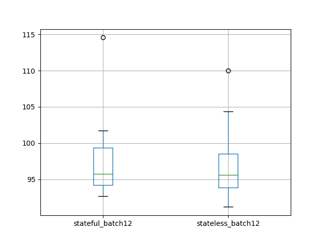
  Box and Whisker Plot of Test RMSE of Stateful vs Stateless with Large Batch Size LSTM Results

  Stateful Resetting vs Stateless

  Another question regarding stateful LSTMs is the best regime to perform resets to state.

  Generally, we would expect that resetting the state after each presentation of the sequence would be a good idea.

  • Expectation 4: Resetting state after each training epoch results in better test performance.

  This raises the question as to the best way to manage state when making predictions. For example, should the network be seeded with state from making predictions on the training dataset first?

  • Expectation 5: Seeding state in the LSTM by making predictions on the training dataset results in better test performance.

  We would also expect that not resetting LSTM state between one-step predictions on the test set would be a good idea.

  • Expectation 6: Not resetting state between one-step predictions on the test set results in better test set performance.

  There is also the question of whether or not resetting state at all is a good idea. In this section, we attempt to tease out answers to these questions.

  We will again use all of the available data and a batch size of 1 for one-step forecasts.

  In summary, we are going to compare the following experimental setups:

  No Seeding:

  • noseed_1: Reset state after each training epoch and not during testing (the stateful results from the first experiment in experiment_stateful.csv).
  • noseed_2: Reset state after each training epoch and after each one-step prediction (experiment_stateful_reset_test.csv).
  • noseed_3: No resets after training or making one-step predictions (experiment_stateful_noreset.csv).

  Seeding:

  • seed_1: Reset state after each training epoch, seed state with one-step predictions on training dataset before making one-step predictions on the test dataset (experiment_stateful_seed_train.csv).
  • seed_2: Reset state after each training epoch, seed state with one-step predictions on training dataset before making one-step predictions on the test dataset and reset state after each one-step prediction on train and test sets (experiment_stateful_seed_train_resets.csv).
  • seed_3: Seed on training dataset before making one-step predictions, no resets during training on predictions (experiment_stateful_seed_train_no_resets.csv).

  The stateful experiment code from the first “A vs A” experiment is used as a base.

  The modifications needed for the various resetting/no-resetting and seeding/no-seeding are listed below.

  We can update the forecast_lstm() function to update after each test by adding a call to reset_states() on the model after each prediction is made. The updated forecast_lstm() function is listed below.

  # make a one-step forecast def forecast_lstm(model, batch_size, X): X = X.reshape(1, 1, len(X)) yhat = model.predict(X, batch_size=batch_size) model.reset_states() return yhat[0,0]

  We can update the fit_lstm() function to not reset after each epoch by removing the call to reset_states(). The complete function is listed below.

  # fit an LSTM network to training data def fit_lstm(train, batch_size, nb_epoch, neurons): X, y = train[:, 0:-1], train[:, -1] X = X.reshape(X.shape[0], 1, X.shape[1]) model = Sequential() model.add(LSTM(neurons, batch_input_shape=(batch_size, X.shape[1], X.shape[2]), stateful=True)) model.add(Dense(1)) model.compile(loss='mean_squared_error', optimizer='adam') for i in range(nb_epoch): model.fit(X, y, epochs=1, batch_size=batch_size, verbose=0, shuffle=False) return model

  We can seed the state of LSTM after training with the state from making predictions on the training dataset by looping through the training dataset and making one-step forecasts. This can be added to the run() function before making one-step forecasts on the test dataset. The updated run() function is listed below.

  # run a repeated experiment def experiment(repeats, series): # transform data to be stationary raw_values = series.values diff_values = difference(raw_values, 1) # transform data to be supervised learning supervised = timeseries_to_supervised(diff_values, 1) supervised_values = supervised.values[1:,:] # split data into train and test-sets train, test = supervised_values[0:-12, :], supervised_values[-12:, :] # transform the scale of the data scaler, train_scaled, test_scaled = scale(train, test) # run experiment error_scores = list() for r in range(repeats): # fit the base model lstm_model = fit_lstm(train_scaled, 1, 1000, 1) # forecast train dataset for i in range(len(train_scaled)): X, y = train_scaled[i, 0:-1], train_scaled[i, -1] yhat = forecast_lstm(lstm_model, 1, X) # forecast test dataset predictions = list() for i in range(len(test_scaled)): # predict X, y = test_scaled[i, 0:-1], test_scaled[i, -1] yhat = forecast_lstm(lstm_model, 1, X) # invert scaling yhat = invert_scale(scaler, X, yhat) # invert differencing yhat = inverse_difference(raw_values, yhat, len(test_scaled)+1-i) # store forecast predictions.append(yhat) # report performance rmse = sqrt(mean_squared_error(raw_values[-12:], predictions)) print('%d) Test RMSE: %.3f' % (r+1, rmse)) error_scores.append(rmse) return error_scores

  This concludes all of the piecewise modifications needed to create the code for these 6 experiments.

  After running these experiments you will have the following results files:

  • experiment_stateful.csv
  • experiment_stateful_reset_test.csv
  • experiment_stateful_noreset.csv
  • experiment_stateful_seed_train.csv
  • experiment_stateful_seed_train_resets.csv
  • experiment_stateful_seed_train_no_resets.csv

  We can now compare the results, using the script below.

  from pandas import DataFrame from pandas import read_csv from matplotlib import pyplot # load results into a dataframe filenames = ['experiment_stateful.csv', 'experiment_stateful_reset_test.csv', 'experiment_stateful_noreset.csv', 'experiment_stateful_seed_train.csv', 'experiment_stateful_seed_train_resets.csv', 'experiment_stateful_seed_train_no_resets.csv'] results = DataFrame() for name in filenames: results[name] = read_csv(name, header=0) results.columns = ['noseed_1', 'noseed_2', 'noseed_3', 'seed_1', 'seed_2', 'seed_3'] # describe all results print(results.describe()) # box and whisker plot results.boxplot() pyplot.show()

  Running the comparison prints descriptive statistics for each set of results.

  Note: Your results may vary given the stochastic nature of the algorithm or evaluation procedure, or differences in numerical precision. Consider running the example a few times and compare the average outcome.

  The results for no seeding suggest perhaps little difference between resetting after each prediction on the test dataset and not. This suggests any state built up from prediction to prediction is not adding value, or that this state is implicitly cleared by the Keras API. This was a surprising result.

  The results on the no-seed case also suggest that having no resets during training results in worse on average performance with larger variance than resetting the state at the end of each epoch. This confirms the expectation that resetting the state at the end of each training epoch is a good practice.

  The average results from the seed experiments suggest that seeding LSTM state with predictions on the training dataset before making predictions on the test dataset is neutral, if not resulting in slightly worse performance.

  Resetting state after each prediction on the train and test sets seem to result in slightly better performance, whereas not resetting state during training or testing seems to result in the best performance.

  These results regarding seeding are surprising, but we should note that the mean values are all within a test RMSE of 5 monthly shampoo sales and could be statistical noise.

  noseed_1    noseed_2    noseed_3      seed_1      seed_2      seed_3 count   10.000000   10.000000   10.000000   10.000000   10.000000   10.000000 mean   103.142903  101.757034  110.441021  105.468200  100.093551   98.766432 std      7.109461   14.584442   24.539690    5.206674    4.157095   11.573366 min     94.052380   91.264712   87.262549   97.683535   95.913385   90.005843 25%     96.765985   93.218929   94.610724  100.974693   96.721924   91.203879 50%    104.376252   96.144883   99.483971  106.036240   98.779770   95.079716 75%    107.753516  105.657586  121.586508  109.829793  103.082791  100.500867 max    114.958430  138.752321  166.527902  112.691046  108.070145  128.261354

  A box and whisker plot is also created to compare the distributions.

  The plot tells the same story as the descriptive statistics. It highlights the increased spread when no resets are used on the stateless LSTM without seeding. It also highlights the general tight spread on the experiments that seed the state of the LSTM with predictions on the training dataset.

  

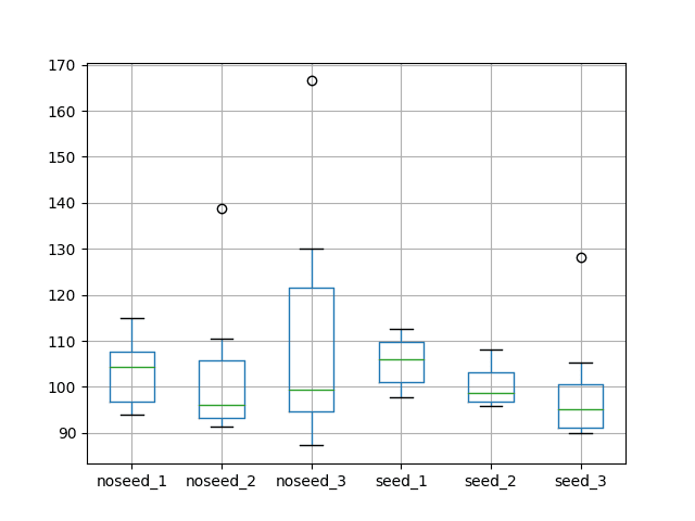
  Box and Whisker Plot of Test RMSE of Reset Regimes in Stateful LSTMs

  Review of Findings

  In this section, we recap the findings throughout this tutorial.

  • 10 repeats of an experiment with the chosen configuration results in some variation in the mean and standard deviation of the test RMSE of about 3 monthly shampoo sales. More repeats would be expected to tighten this up.
  • The stateless LSTM with the same configuration may perform better on this problem than the stateful version.
  • Not shuffling training patterns with the stateless LSTM may result in slightly better performance.
  • When a large batch size is used, a stateful LSTM can be simulated with a stateless LSTM.
  • Resetting state when making one-step predictions with a stateful LSTM may improve performance on the test set.
  • Seeding state in a stateful LSTM by making predictions on the training dataset before making predictions on the test set does not result in an obvious improvement in performance on the test set.
  • Fitting a stateful LSTM and seeding it on the training dataset and not performing any resetting of state during training or prediction may result in better performance on the test set.

  It must be noted that these findings should be made more robust by increasing the number of repeats of each experiment and confirming the differences are significant using statistical significance tests.

  It should also be noted that these results apply to this specific problem, the way it was framed, and the chosen LSTM configuration parameters including topology, batch size, and training epochs.

  Summary

  In this tutorial, you discovered how to investigate the impact of using stateful vs stateless LSTM networks for time series forecasting in Python with Keras.

  Specifically, you learned:

  • How to compare stateless vs stateful LSTM networks for time series forecasting.
  • How to confirm the equivalence of stateless LSTMs and stateful LSTMs with a large batch size.
  • How to evaluate the impact of when LSTM state is reset during training and making predictions with LSTM networks for time series forecasting.

  Do you have any questions? Ask your questions in the comments and I will do my best to answer.