How to Make Predictions for Time Series Forecasting with Python

 Selecting a time series forecasting model is just the beginning.

Using the chosen model in practice can pose challenges, including data transformations and storing the model parameters on disk.

In this tutorial, you will discover how to finalize a time series forecasting model and use it to make predictions in Python.

After completing this tutorial, you will know:

• How to finalize a model and save it and required data to file.
• How to load a finalized model from file and use it to make a prediction.
• How to update data associated with a finalized model in order to make subsequent predictions.

  Process for Making a Prediction

  A lot is written about how to tune specific time series forecasting models, but little help is given to how to use a model to make predictions.

  Once you can build and tune forecast models for your data, the process of making a prediction involves the following steps:

  1. Model Selection. This is where you choose a model and gather evidence and support to defend the decision.
  2. Model Finalization. The chosen model is trained on all available data and saved to file for later use.
  3. Forecasting. The saved model is loaded and used to make a forecast.
  4. Model Update. Elements of the model are updated in the presence of new observations.

  We will take a look at each of these elements in this tutorial, with a focus on saving and loading the model to and from file and using a loaded model to make predictions.

  Before we dive in, let’s first look at a standard univariate dataset that we can use as the context for this tutorial.

  Stop learning Time Series Forecasting the slow way!

  Take my free 7-day email course and discover how to get started (with sample code).

  Click to sign-up and also get a free PDF Ebook version of the course.

  Daily Female Births Dataset

  This dataset describes the number of daily female births in California in 1959.

  The units are a count and there are 365 observations. The source of the dataset is credited to Newton (1988).

  • Download the dataset.

  Download the dataset and place it in your current working directory with the filename “daily-total-female-births.csv“.

  We can load the dataset as a Pandas series. The snippet below loads and plots the dataset.

  from pandas import read_csv from matplotlib import pyplot series = read_csv('daily-total-female-births.csv', header=0, index_col=0) print(series.head()) series.plot() pyplot.show()

  Running the example prints the first 5 rows of the dataset.

  Date 1959-01-01    35 1959-01-02    32 1959-01-03    30 1959-01-04    31 1959-01-05    44

  The series is then graphed as a line plot.

  

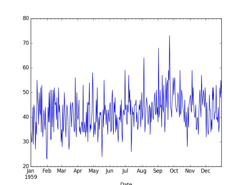
  Daily Female Birth Dataset Line Plot

  1. Select Time Series Forecast Model

  You must select a model.

  This is where the bulk of the effort will be in preparing the data, performing analysis, and ultimately selecting a model and model hyperparameters that best capture the relationships in the data.

  In this case, we can arbitrarily select an autoregression model (AR) with a lag of 6 on the differenced dataset.

  We can demonstrate this model below.

  First, the data is transformed by differencing, with each observation transformed as:

  value(t) = obs(t) - obs(t - 1)

  Next, the AR(6) model is trained on 66% of the historical data. The regression coefficients learned by the model are extracted and used to make predictions in a rolling manner across the test dataset.

  As each time step in the test dataset is executed, the prediction is made using the coefficients and stored. The actual observation for the time step is then made available and stored to be used as a lag variable for future predictions.

  # fit and evaluate an AR model from pandas import read_csv from matplotlib import pyplot from statsmodels.tsa.ar_model import AutoReg from sklearn.metrics import mean_squared_error import numpy from math import sqrt   # create a difference transform of the dataset def difference(dataset): diff = list() for i in range(1, len(dataset)): value = dataset[i] - dataset[i - 1] diff.append(value) return numpy.array(diff)   # Make a prediction give regression coefficients and lag obs def predict(coef, history): yhat = coef[0] for i in range(1, len(coef)): yhat += coef[i] * history[-i] return yhat   series = read_csv('daily-total-female-births.csv', header=0, index_col=0, parse_dates=True, squeeze=True) # split dataset X = difference(series.values) size = int(len(X) * 0.66) train, test = X[0:size], X[size:] # train autoregression window = 6 model = AutoReg(train, lags=6) model_fit = model.fit() coef = model_fit.params # walk forward over time steps in test history = [train[i] for i in range(len(train))] predictions = list() for t in range(len(test)): yhat = predict(coef, history) obs = test[t] predictions.append(yhat) history.append(obs) rmse = sqrt(mean_squared_error(test, predictions)) print('Test RMSE: %.3f' % rmse) # plot pyplot.plot(test) pyplot.plot(predictions, color='red') pyplot.show()

  Running the example first prints the Root Mean Squared Error (RMSE) of the predictions, which is about 7 births on average.

  This is how well we expect the model to perform on average when making forecasts on new data.

  Test RMSE: 7.259

  Finally, a graph is created showing the actual observations in the test dataset (blue) compared to the predictions (red).

  

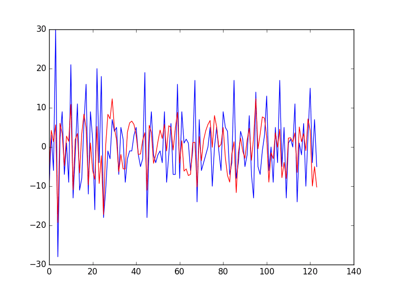
  Predictions vs Actual Daily Female Birth Dataset Line Plot

  This may not be the very best possible model we could develop on this problem, but it is reasonable and skillful.

  2. Finalize and Save Time Series Forecast Model

  Once the model is selected, we must finalize it.

  This means save the salient information learned by the model so that we do not have to re-create it every time a prediction is needed.

  This involves first training the model on all available data and then saving the model to file.

  The statsmodels implementations of time series models do provide built-in capability to save and load models by calling save() and load() on the fit AutoRegResults object.

  For example, the code below will train an AR(6) model on the entire Female Births dataset and save it using the built-in save() function, which will essentially pickle the AutoRegResults object.

  The differenced training data must also be saved, both the for the lag variables needed to make a prediction, and for knowledge of the number of observations seen, required by the predict() function of the AutoRegResults object.

  Finally, we need to be able to transform the differenced dataset back into the original form. To do this, we must keep track of the last actual observation. This is so that the predicted differenced value can be added to it.

  # fit an AR model and save the whole model to file from pandas import read_csv from statsmodels.tsa.ar_model import AutoReg import numpy   # create a difference transform of the dataset def difference(dataset): diff = list() for i in range(1, len(dataset)): value = dataset[i] - dataset[i - 1] diff.append(value) return numpy.array(diff)   # load dataset series = read_csv('daily-total-female-births.csv', header=0, index_col=0, parse_dates=True, squeeze=True) X = difference(series.values) # fit model model = AutoReg(X, lags=6) model_fit = model.fit() # save model to file model_fit.save('ar_model.pkl') # save the differenced dataset numpy.save('ar_data.npy', X) # save the last ob numpy.save('ar_obs.npy', [series.values[-1]])

  This code will create a file ar_model.pkl that you can load later and use to make predictions.

  The entire training dataset is saved as ar_data.npy and the last observation is saved in the file ar_obs.npy as an array with one item.

  The NumPy save() function is used to save the differenced training data and the observation. The load() function can then be used to load these arrays later.

  The snippet below will load the model, differenced data, and last observation.

  # load the AR model from file from statsmodels.tsa.ar_model import AutoRegResults import numpy loaded = AutoRegResults.load('ar_model.pkl') print(loaded.params) data = numpy.load('ar_data.npy') last_ob = numpy.load('ar_obs.npy') print(last_ob)

  Running the example prints the coefficients and the last observation.

  [ 0.12129822 -0.75275857 -0.612367   -0.51097172 -0.4176669  -0.32116469 -0.23412997] [50]

  I think this is good for most cases, but is also pretty heavy. You are subject to changes to the statsmodels API.

  My preference is to work with the coefficients of the model directly, as in the case above, evaluating the model using a rolling forecast.

  In this case, you could simply store the model coefficients and later load them and make predictions.

  The example below saves just the coefficients from the model, as well as the minimum differenced lag values required to make the next prediction and the last observation needed to transform the next prediction made.

  # fit an AR model and manually save coefficients to file from pandas import read_csv from statsmodels.tsa.ar_model import AutoReg import numpy   # create a difference transform of the dataset def difference(dataset): diff = list() for i in range(1, len(dataset)): value = dataset[i] - dataset[i - 1] diff.append(value) return numpy.array(diff)   # load dataset series = read_csv('daily-total-female-births.csv', header=0, index_col=0, parse_dates=True, squeeze=True) X = difference(series.values) # fit model window_size = 6 model = AutoReg(X, lags=window_size) model_fit = model.fit() # save coefficients coef = model_fit.params numpy.save('man_model.npy', coef) # save lag lag = X[-window_size:] numpy.save('man_data.npy', lag) # save the last ob numpy.save('man_obs.npy', [series.values[-1]])

  The coefficients are saved in the local file man_model.npy, the lag history is saved in the file man_data.npy, and the last observation is saved in the file man_obs.npy.

  These values can then be loaded again as follows:

  # load the manually saved model from file import numpy coef = numpy.load('man_model.npy') print(coef) lag = numpy.load('man_data.npy') print(lag) last_ob = numpy.load('man_obs.npy') print(last_ob)

  Running this example prints the loaded data for review. We can see the coefficients and last observation match the output from the previous example.

  [ 0.12129822 -0.75275857 -0.612367   -0.51097172 -0.4176669  -0.32116469 -0.23412997] [-10   3  15  -4   7  -5] [50]

  Now that we know how to save a finalized model, we can use it to make forecasts.

  3. Make a Time Series Forecast

  Making a forecast involves loading the saved model and estimating the observation at the next time step.

  If the AutoRegResults object was serialized, we can use the predict() function to predict the next time period.

  The example below shows how the next time period can be predicted.

  The model, training data, and last observation are loaded from file.

  The period is specified to the predict() function as the next time index after the end of the training data set. This index may be stored directly in a file instead of storing the entire training data, which may be an efficiency.

  The prediction is made, which is in the context of the differenced dataset. To turn the prediction back into the original units, it must be added to the last known observation.

  # load AR model from file and make a one-step prediction from statsmodels.tsa.ar_model import AutoRegResults import numpy # load model model = AutoRegResults.load('ar_model.pkl') data = numpy.load('ar_data.npy') last_ob = numpy.load('ar_obs.npy') # make prediction predictions = model.predict(start=len(data), end=len(data)) # transform prediction yhat = predictions[0] + last_ob[0] print('Prediction: %f' % yhat)

  Running the example prints the prediction.

  Prediction: 46.755211

  We can also use a similar trick to load the raw coefficients and make a manual prediction.
  The complete example is listed below.

  # load a coefficients and from file and make a manual prediction import numpy   def predict(coef, history): yhat = coef[0] for i in range(1, len(coef)): yhat += coef[i] * history[-i] return yhat   # load model coef = numpy.load('man_model.npy') lag = numpy.load('man_data.npy') last_ob = numpy.load('man_obs.npy') # make prediction prediction = predict(coef, lag) # transform prediction yhat = prediction + last_ob[0] print('Prediction: %f' % yhat)

  Running the example, we achieve the same prediction as we would expect, given the underlying model and method for making the prediction are the same.

  Prediction: 46.755211

  4. Update Forecast Model

  Our work is not done.

  Once the next real observation is made available, we must update the data associated with the model.

  Specifically, we must update:

  1. The differenced training dataset used as inputs to make the subsequent prediction.
  2. The last observation, providing a context for the predicted differenced value.

  Let’s assume the next actual observation in the series was 48.
  The new observation must first be differenced with the last observation. It can then be stored in the list of differenced observations. Finally, the value can be stored as the last observation.

  In the case of the stored AR model, we can update the ar_data.npy and ar_obs.npy files. The complete example is listed below:

  # update the data for the AR model with a new obs import numpy # get real observation observation = 48 # load the saved data data = numpy.load('ar_data.npy') last_ob = numpy.load('ar_obs.npy') # update and save differenced observation diffed = observation - last_ob[0] data = numpy.append(data, [diffed], axis=0) numpy.save('ar_data.npy', data) # update and save real observation last_ob[0] = observation numpy.save('ar_obs.npy', last_ob)

  We can make the same changes for the data files for the manual case. Specifically, we can update the man_data.npy and man_obs.npy respectively.

  The complete example is listed below.

  # update the data for the manual model with a new obs import numpy # get real observation observation = 48 # update and save differenced observation lag = numpy.load('man_data.npy') last_ob = numpy.load('man_obs.npy') diffed = observation - last_ob[0] lag = numpy.append(lag[1:], [diffed], axis=0) numpy.save('man_data.npy', lag) # update and save real observation last_ob[0] = observation numpy.save('man_obs.npy', last_ob)

  We have focused on one-step forecasts.

  These methods would work just as easily for multi-step forecasts, by using the model repetitively and using forecasts of previous time steps as input lag values to predict observations for subsequent time steps.

  Consider Storing All Observations

  Generally, it is a good idea to keep track of all the observations.

  This will allow you to:

  • Provide a context for further time series analysis to understand new changes in the data.
  • Train a new model in the future on the most recent data.
  • Back-test new and different models to see if performance can be improved.

  For small applications, perhaps you could store the raw observations in a file alongside your model.

  It may also be desirable to store the model coefficients and required lag data and last observation in plain text for easy review.

  For larger applications, perhaps a database system could be used to store the observations.

  Summary

  In this tutorial, you discovered how to finalize a time series model and use it to make predictions with Python.

  Specifically, you learned:

  • How to save a time series forecast model to file.
  • How to load a saved time series forecast from file and make a prediction.
  • How to update a time series forecast model with new observations.

  Do you have any questions?
  Ask your questions in the comments below and I will do my best to answer.