Time series forecasting is a process, and the only way to get good forecasts is to practice this process.
In this tutorial, you will discover how to forecast the annual water usage in Baltimore with Python.
Working through this tutorial will provide you with a framework for the steps and the tools for working through your own time series forecasting problems.
After completing this tutorial, you will know:
- How to confirm your Python environment and carefully define a time series forecasting problem.
- How to create a test harness for evaluating models, develop a baseline forecast, and better understand your problem with the tools of time series analysis.
- How to develop an autoregressive integrated moving average model,
save it to file, and later load it to make predictions for new time
steps.
Overview
In this tutorial, we will work through a time series forecasting project from end-to-end, from downloading the dataset and defining the problem to training a final model and making predictions.
This project is not exhaustive, but shows how you can get good results quickly by working through a time series forecasting problem systematically.
The steps of this project that we will work through are as follows.
- Environment.
- Problem Description.
- Test Harness.
- Persistence.
- Data Analysis.
- ARIMA Models.
- Model Validation.
This will provide a template for working through a time series prediction problem that you can use on your own dataset.
Stop learning Time Series Forecasting the slow way!
Take my free 7-day email course and discover how to get started (with sample code).
Click to sign-up and also get a free PDF Ebook version of the course.
1. Environment
This tutorial assumes an installed and working SciPy environment and dependencies, including:
- SciPy
- NumPy
- Matplotlib
- Pandas
- scikit-learn
- statsmodels
If you need help installing Python and the SciPy environment on your workstation, consider the Anaconda distribution that manages much of it for you.
This script will help you check your installed versions of these libraries.
The results on my workstation used to write this tutorial are as follows:
2. Problem Description
The problem is to predict annual water usage.
The dataset provides the annual water usage in Baltimore from 1885 to 1963, or 79 years of data.
The values are in the units of liters per capita per day, and there are 79 observations.
The dataset is credited to Hipel and McLeod, 1994.
Download the dataset as a CSV file and place it in your current working directory with the filename “water.csv“.
3. Test Harness
We must develop a test harness to investigate the data and evaluate candidate models.
This involves two steps:
- Defining a Validation Dataset.
- Developing a Method for Model Evaluation.
3.1 Validation Dataset
The dataset is not current. This means that we cannot easily collect updated data to validate the model.
Therefore, we will pretend that it is 1953 and withhold the last 10 years of data from analysis and model selection.
This final decade of data will be used to validate the final model.
The code below will load the dataset as a Pandas Series and split into two, one for model development (dataset.csv) and the other for validation (validation.csv).
Running the example creates two files and prints the number of observations in each.
The specific contents of these files are:
- dataset.csv: Observations from 1885 to 1953 (69 observations).
- validation.csv: Observations from 1954 to 1963 (10 observations).
The validation dataset is about 12% of the original dataset.
Note that the saved datasets do not have a header line, therefore we do not need to cater to this when working with these files later.
3.2. Model Evaluation
Model evaluation will only be performed on the data in dataset.csv prepared in the previous section.
Model evaluation involves two elements:
- Performance Measure.
- Test Strategy.
3.2.1 Performance Measure
We will evaluate the performance of predictions using the root mean squared error (RMSE). This will give more weight to predictions that are grossly wrong and will have the same units as the original data.
Any transforms to the data must be reversed before the RMSE is calculated and reported to make the performance between different methods directly comparable.
We can calculate the RMSE using the helper function from the scikit-learn library mean_squared_error() that calculates the mean squared error between a list of expected values (the test set) and the list of predictions. We can then take the square root of this value to give us a RMSE score.
For example:
3.2.2 Test Strategy
Candidate models will be evaluated using walk-forward validation.
This is because a rolling-forecast type model is required from the problem definition. This is where one-step forecasts are needed given all available data.
The walk-forward validation will work as follows:
- The first 50% of the dataset will be held back to train the model.
- The remaining 50% of the dataset will be iterated and test the model.
- For each step in the test dataset:
- A model will be trained.
- A one-step prediction made and the prediction stored for later evaluation.
- The actual observation from the test dataset will be added to the training dataset for the next iteration.
- The predictions made during the enumeration of the test dataset will be evaluated and an RMSE score reported.
Given the small size of the data, we will allow a model to be re-trained given all available data prior to each prediction.
We can write the code for the test harness using simple NumPy and Python code.
Firstly, we can split the dataset into train and test sets directly. We’re careful to always convert a loaded dataset to float32 in case the loaded data still has some String or Integer data types.
Next, we can iterate over the time steps in the test dataset. The train dataset is stored in a Python list as we need to easily append a new observation each iteration and NumPy array concatenation feels like overkill.
The prediction made by the model is called yhat for convention, as the outcome or observation is referred to as y and yhat (a ‘y‘ with a mark above) is the mathematical notation for the prediction of the y variable.
The prediction and observation are printed each observation for a sanity check prediction in case there are issues with the model.
4. Persistence
The first step before getting bogged down in data analysis and modeling is to establish a baseline of performance.
This will provide both a template for evaluating models using the proposed test harness and a performance measure by which all more elaborate predictive models can be compared.
The baseline prediction for time series forecasting is called the naive forecast, or persistence.
This is where the observation from the previous time step is used as the prediction for the observation at the next time step.
We can plug this directly into the test harness defined in the previous section.
The complete code listing is provided below.
Running the test harness prints the prediction and observation for each iteration of the test dataset.
The example ends by printing the RMSE for the model.
In this case, we can see that the persistence model achieved an RMSE of 21.975. This means that on average, the model was wrong by about 22 liters per capita per day for each prediction made.
We now have a baseline prediction method and performance; now we can start digging into our data.
5. Data Analysis
We can use summary statistics and plots of the data to quickly learn more about the structure of the prediction problem.
In this section, we will look at the data from four perspectives:
- Summary Statistics.
- Line Plot.
- Density Plots.
- Box and Whisker Plot.
5.1. Summary Statistics
Summary statistics provide a quick look at the limits of observed values. It can help to get a quick idea of what we are working with.
The example below calculates and prints summary statistics for the time series.
Running the example provides a number of summary statistics to review.
Some observations from these statistics include:
- The number of observations (count) matches our expectation, meaning we are handling the data correctly.
- The mean is about 500, which we might consider our level in this series.
- The standard deviation and percentiles suggest a reasonably tight spread around the mean.
5.2. Line Plot
A line plot of a time series dataset can provide a lot of insight into the problem.
The example below creates and shows a line plot of the dataset.
Run the example and review the plot. Note any obvious temporal structures in the series.
Some observations from the plot include:
- There looks to be an increasing trend in water usage over time.
- There do not appear to be any obvious outliers, although there are some large fluctuations.
- There is a downward trend for the last few years of the series.
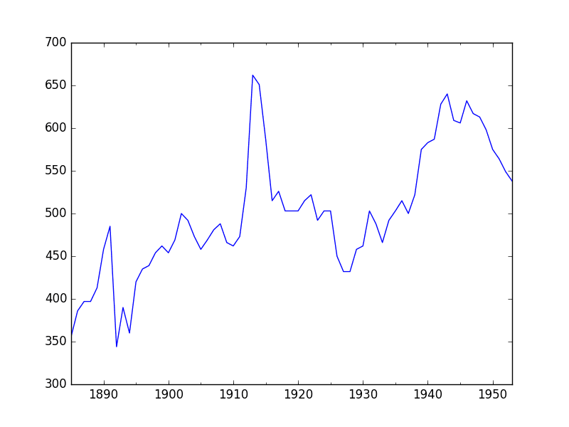
Annual Water Usage Line Plot
There may be some benefit in explicitly modeling the trend component and removing it. You may also explore using differencing with one or two levels in order to make the series stationary.
5.3. Density Plot
Reviewing plots of the density of observations can provide further insight into the structure of the data.
The example below creates a histogram and density plot of the observations without any temporal structure.
Run the example and review the plots.
Some observations from the plots include:
- The distribution is not Gaussian, but is pretty close.
- The distribution has a long right tail and may suggest an exponential distribution or a double Gaussian.
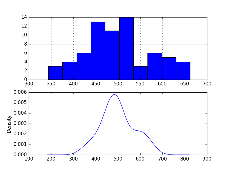
Annual Water Usage Density Plots
This suggests it may be worth exploring some power transforms of the data prior to modeling.
5.4. Box and Whisker Plots
We can group the annual data by decade and get an idea of the spread of observations for each decade and how this may be changing.
We do expect to see some trend (increasing mean or median), but it may be interesting to see how the rest of the distribution may be changing.
The example below groups the observations by decade and creates one box and whisker plot for each decade of observations. The last decade only contains 9 years and may not be a useful comparison with the other decades. Therefore only data between 1885 and 1944 was plotted.
Running the example creates 6 box and whisker plots side-by-side, one for the 6 decades of selected data.
Some observations from reviewing the plot include:
- The median values for each year (red line) may show an increasing trend that may not be linear.
- The spread, or middle 50% of the data (blue boxes), does show some variability.
- There maybe outliers in some decades (crosses outside of the box and whiskers).
- The second to last decade seems to have a lower average consumption, perhaps related to the first world war.
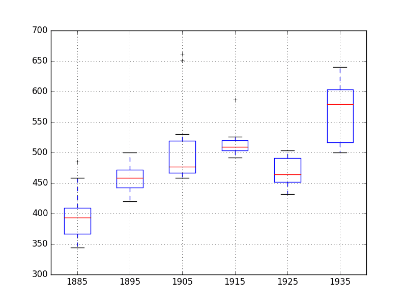
Annual Water Usage Box and Whisker Plots
This yearly view of the data is an interesting avenue and could be pursued further by looking at summary statistics from decade-to-decade and changes in summary statistics.
6. ARIMA Models
In this section, we will develop Autoregressive Integrated Moving Average or ARIMA models for the problem.
We will approach modeling by both manual and automatic configuration of the ARIMA model. This will be followed by a third step of investigating the residual errors of the chosen model.
As such, this section is broken down into 3 steps:
- Manually Configure the ARIMA.
- Automatically Configure the ARIMA.
- Review Residual Errors.
6.1 Manually Configured ARIMA
The ARIMA(p,d,q) model requires three parameters and is traditionally configured manually.
Analysis of the time series data assumes that we are working with a stationary time series.
The time series is likely non-stationary. We can make it stationary by first differencing the series and using a statistical test to confirm that the result is stationary.
The example below creates a stationary version of the series and saves it to file stationary.csv.
Running the example outputs the result of a statistical significance test of whether the differenced series is stationary. Specifically, the augmented Dickey-Fuller test.
The results show that the test statistic value -6.126719 is smaller than the critical value at 1% of -3.534. This suggests that we can reject the null hypothesis with a significance level of less than 1% (i.e. a low probability that the result is a statistical fluke).
Rejecting the null hypothesis means that the process has no unit root, and in turn that the time series is stationary or does not have time-dependent structure.
This suggests that at least one level of differencing is required. The d parameter in our ARIMA model should at least be a value of 1.
A plot of the differenced data is also created. It suggests that this has indeed removed the increasing trend.
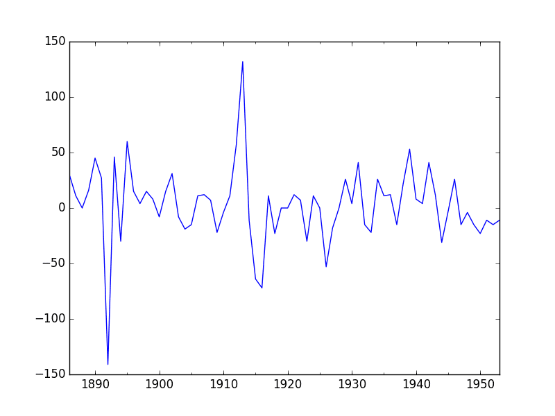
Differenced Annual Water Usage Dataset
The next first step is to select the lag values for the Autoregression (AR) and Moving Average (MA) parameters, p and q respectively.
We can do this by reviewing Autocorrelation Function (ACF) and Partial Autocorrelation Function (PACF) plots.
The example below creates ACF and PACF plots for the series.
Run the example and review the plots for insights into how to set the p and q variables for the ARIMA model.
Below are some observations from the plots.
- The ACF shows no significant lags.
- The PACF also shows no significant lags.
A good starting point for the p and q values is also 0.
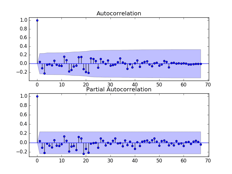
ACF and PACF Plots of Stationary Annual Water Usage Dataset
This quick analysis suggests an ARIMA(0,1,0) on the raw data may be a good starting point.
This is in fact a persistence model. The complete example is listed below.
Running this example results in an RMSE of 22.311, which is slightly higher than the persistence model above.
This may be because of the details of the ARIMA implementation, such as an automatic trend constant that is calculated and added.
6.2 Grid Search ARIMA Hyperparameters
The ACF and PACF plots suggest that we cannot do better than a persistence model on this dataset.
To confirm this analysis, we can grid search a suite of ARIMA hyperparameters and check that no models result in better out of sample RMSE performance.
In this section, we will search values of p, d, and q for combinations (skipping those that fail to converge), and find the combination that results in the best performance. We will use a grid search to explore all combinations in a subset of integer values.
Specifically, we will search all combinations of the following parameters:
- p: 0 to 4.
- d: 0 to 2.
- q: 0 to 4.
This is (5 * 3 * 5), or 300 potential runs of the test harness, and will take some time to execute.
The complete worked example with the grid search version of the test harness is listed below.
Running the example runs through all combinations and reports the results on those that converge without error. The example takes a little over 2 minutes to run on modern hardware.
The results show that the best configuration discovered was ARIMA(2, 1, 0) with an RMSE of 21.733, slightly lower than the manual persistence model tested earlier, but may or may not be significantly different.
We will select this ARIMA(2, 1, 0) model going forward.
6.3 Review Residual Errors
A good final check of a model is to review residual forecast errors.
Ideally, the distribution of residual errors should be a Gaussian with a zero mean.
We can check this by using summary statistics and plots to investigate the residual errors from the ARIMA(2, 1, 0) model. The example below calculates and summarizes the residual forecast errors.
Running the example first describes the distribution of the residuals.
We can see that the distribution has a right shift and that the mean is non-zero at 1.081624.
This is perhaps a sign that the predictions are biased.
The distribution of residual errors is also plotted.
The graphs suggest a Gaussian-like distribution with a longer right tail, providing further evidence that perhaps a power transform might be worth exploring.
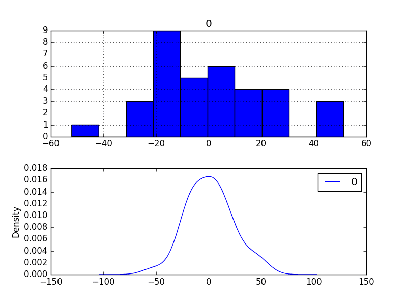
Residual Forecast Errors Density Plots
We could use this information to bias-correct predictions by adding the mean residual error of 1.081624 to each forecast made.
The example below performs this bias-correction.
The performance of the predictions is improved very slightly from 21.733 to 21.706, which may or may not be significant.
The summary of the forecast residual errors shows that the mean was indeed moved to a value very close to zero.
Finally, density plots of the residual error do show a small shift towards zero.
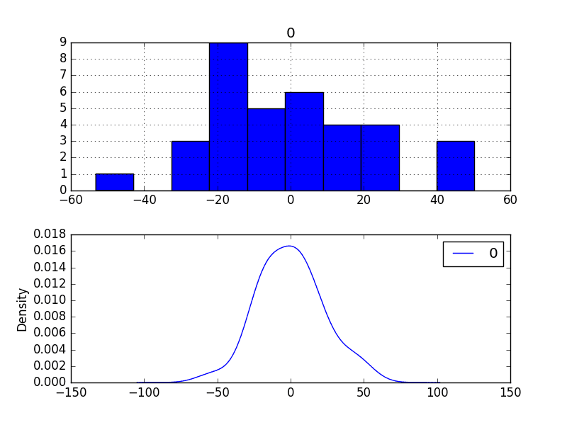
Bias-Corrected Residual Forecast Errors Density Plots
It is debatable whether this bias correction is worth it, but we will use it for now.
7. Model Validation
After models have been developed and a final model selected, it must be validated and finalized.
Validation is an optional part of the process, but one that provides a ‘last check’ to ensure we have not fooled or misled ourselves.
This section includes the following steps:
- Finalize Model: Train and save the final model.
- Make Prediction: Load the finalized model and make a prediction.
- Validate Model: Load and validate the final model.
7.1 Finalize Model
Finalizing the model involves fitting an ARIMA model on the entire dataset, in this case, on a transformed version of the entire dataset.
Once fit, the model can be saved to file for later use.
The example below trains an ARIMA(2,1,0) model on the dataset and saves the whole fit object and the bias to file.
The example below saves the fit model to file in the correct state so that it can be loaded successfully later.
Running the example creates two local files:
- model.pkl This is the ARIMAResult object from the call to ARIMA.fit(). This includes the coefficients and all other internal data returned when fitting the model.
- model_bias.npy This is the bias value stored as a one-row, one-column NumPy array.
7.2 Make Prediction
A natural case may be to load the model and make a single forecast.
This is relatively straightforward and involves restoring the saved model and the bias and calling the forecast() function.
The example below loads the model, makes a prediction for the next time step, and prints the prediction.
Running the example prints the prediction of about 540.
If we peek inside validation.csv, we can see that the value on the first row for the next time period is 568. The prediction is in the right ballpark.
7.3 Validate Model
We can load the model and use it in a pretend operational manner.
In the test harness section, we saved the final 10 years of the original dataset in a separate file to validate the final model.
We can load this validation.csv file now and use it to see how well our model really is on “unseen” data.
There are two ways we might proceed:
- Load the model and use it to forecast the next 10 years. The forecast beyond the first one or two years will quickly start to degrade in skill.
- Load the model and use it in a rolling-forecast manner, updating the transform and model for each time step. This is the preferred method as it is how one would use this model in practice as it would achieve the best performance.
As with model evaluation in the previous sections, we will make predictions in a rolling-forecast manner. This means that we will step over lead times in the validation dataset and take the observations as an update to the history.
Running the example prints each prediction and expected value for the time steps in the validation dataset.
The final RMSE for the validation period is predicted at 16 liters per capita per day. This is not too different from the expected error of 21, but I would expect that it is also not too different from a simple persistence model.
A plot of the predictions compared to the validation dataset is also provided.
The forecast does have the characteristics of a persistence forecast. This suggests that although this time series does have an obvious trend, it is still a reasonably difficult problem.
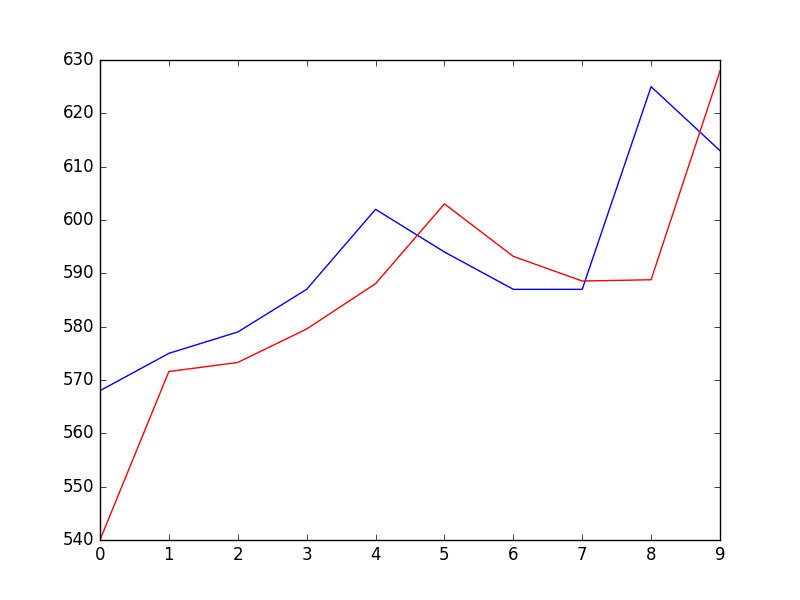
Plot of Forecast for Validation Dataset
Summary
In this tutorial, you discovered the steps and the tools for a time series forecasting project with Python.
We covered a lot of ground in this tutorial; specifically:
- How to develop a test harness with a performance measure and evaluation method and how to quickly develop a baseline forecast and skill.
- How to use time series analysis to raise ideas for how to best model the forecast problem.
- How to develop an ARIMA model, save it, and later load it to make predictions on new data.
How did you do? Do you have any questions about this tutorial?
Ask your questions in the comments below and I will do my best to answer.


No comments:
Post a Comment