How to Identify and Remove Seasonality from Time Series Data with Python

 Time series datasets can contain a seasonal component.

This is a cycle that repeats over time, such as monthly or yearly. This repeating cycle may obscure the signal that we wish to model when forecasting, and in turn may provide a strong signal to our predictive models.

In this tutorial, you will discover how to identify and correct for seasonality in time series data with Python.

After completing this tutorial, you will know:

• The definition of seasonality in time series and the opportunity it provides for forecasting with machine learning methods.
• How to use the difference method to create a seasonally adjusted time series of daily temperature data.
• How to model the seasonal component directly and explicitly subtract it from observations.

Kick-start your project with my new book Time Series Forecasting With Python, including step-by-step tutorials and the Python source code files for all examples.

Let’s get started.

• Updated Apr/2019: Updated the link to dataset.
• Updated Aug/2019: Updated data loading to use new API.

How to Identify and Remove Seasonality from Time Series Data with Python
Photo by naturalflow, some rights reserved.

Seasonality in Time Series

Time series data may contain seasonal variation.

Seasonal variation, or seasonality, are cycles that repeat regularly over time.

A repeating pattern within each year is known as seasonal variation, although the term is applied more generally to repeating patterns within any fixed period.

— Page 6, Introductory Time Series with R

A cycle structure in a time series may or may not be seasonal. If it consistently repeats at the same frequency, it is seasonal, otherwise it is not seasonal and is called a cycle.

Benefits to Machine Learning

Understanding the seasonal component in time series can improve the performance of modeling with machine learning.

This can happen in two main ways:

• Clearer Signal: Identifying and removing the seasonal component from the time series can result in a clearer relationship between input and output variables.
• More Information: Additional information about the seasonal component of the time series can provide new information to improve model performance.

Both approaches may be useful on a project. Modeling seasonality and removing it from the time series may occur during data cleaning and preparation.

Extracting seasonal information and providing it as input features, either directly or in summary form, may occur during feature extraction and feature engineering activities.

Types of Seasonality

There are many types of seasonality; for example:

• Time of Day.
• Daily.
• Weekly.
• Monthly.
• Yearly.

As such, identifying whether there is a seasonality component in your time series problem is subjective.

The simplest approach to determining if there is an aspect of seasonality is to plot and review your data, perhaps at different scales and with the addition of trend lines.

Removing Seasonality

Once seasonality is identified, it can be modeled.

The model of seasonality can be removed from the time series. This process is called Seasonal Adjustment, or Deseasonalizing.

A time series where the seasonal component has been removed is called seasonal stationary. A time series with a clear seasonal component is referred to as non-stationary.

There are sophisticated methods to study and extract seasonality from time series in the field of Time Series Analysis. As we are primarily interested in predictive modeling and time series forecasting, we are limited to methods that can be developed on historical data and available when making predictions on new data.

In this tutorial, we will look at two methods for making seasonal adjustments on a classical meteorological-type problem of daily temperatures with a strong additive seasonal component. Next, let’s take a look at the dataset we will use in this tutorial.

Minimum Daily Temperatures Dataset

This dataset describes the minimum daily temperatures over 10 years (1981-1990) in the city Melbourne, Australia.

The units are in degrees Celsius and there are 3,650 observations. The source of the data is credited as the Australian Bureau of Meteorology.

• Download the dataset.

Below is a sample of the first 5 rows of data, including the header row.

"Date","Temperature" "1981-01-01",20.7 "1981-01-02",17.9 "1981-01-03",18.8 "1981-01-04",14.6 "1981-01-05",15.8

Below is a plot of the entire dataset where you can download the dataset and learn more about it.

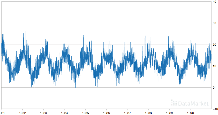
Minimum Daily Temperatures

The dataset shows a strong seasonality component and has a nice, fine-grained detail to work with.

Load the Minimum Daily Temperatures Dataset

Download the Minimum Daily Temperatures dataset and place it in the current working directory with the filename “daily-minimum-temperatures.csv“.

• Download the dataset.

The code below will load and plot the dataset.

from pandas import read_csv from matplotlib import pyplot series = read_csv('daily-minimum-temperatures.csv', header=0, index_col=0) series.plot() pyplot.show()

Running the example creates the following plot of the dataset.

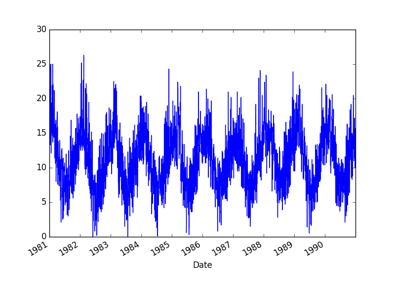
Minimum Daily Temperature Dataset

Seasonal Adjustment with Differencing

A simple way to correct for a seasonal component is to use differencing.

If there is a seasonal component at the level of one week, then we can remove it on an observation today by subtracting the value from last week.

In the case of the Minimum Daily Temperatures dataset, it looks like we have a seasonal component each year showing swing from summer to winter.

We can subtract the daily minimum temperature from the same day last year to correct for seasonality. This would require special handling of February 29th in leap years and would mean that the first year of data would not be available for modeling.

Below is an example of using the difference method on the daily data in Python.

from pandas import read_csv from matplotlib import pyplot series = read_csv('daily-minimum-temperatures.csv', header=0, index_col=0) X = series.values diff = list() days_in_year = 365 for i in range(days_in_year, len(X)): value = X[i] - X[i - days_in_year] diff.append(value) pyplot.plot(diff) pyplot.show()

Running this example creates a new seasonally adjusted dataset and plots the result.

Differencing Sesaonal Adjusted Minimum Daily Temperature

There are two leap years in our dataset (1984 and 1988). They are not explicitly handled; this means that observations in March 1984 onwards the offset are wrong by one day, and after March 1988, the offsets are wrong by two days.

One option is to update the code example to be leap-day aware.

Another option is to consider that the temperature within any given period of the year is probably stable. Perhaps over a few weeks. We can shortcut this idea and consider all temperatures within a calendar month to be stable.

An improved model may be to subtract the average temperature from the same calendar month in the previous year, rather than the same day.

We can start off by resampling the dataset to a monthly average minimum temperature.

from pandas import read_csv from matplotlib import pyplot series = read_csv('daily-minimum-temperatures.csv', header=0, index_col=0) resample = series.resample('M') monthly_mean = resample.mean() print(monthly_mean.head(13)) monthly_mean.plot() pyplot.show()

Running this example prints the first 13 months of average monthly minimum temperatures.

Date 1981-01-31 17.712903 1981-02-28 17.678571 1981-03-31 13.500000 1981-04-30 12.356667 1981-05-31 9.490323 1981-06-30 7.306667 1981-07-31 7.577419 1981-08-31 7.238710 1981-09-30 10.143333 1981-10-31 10.087097 1981-11-30 11.890000 1981-12-31 13.680645 1982-01-31 16.567742

It also plots the monthly data, clearly showing the seasonality of the dataset.

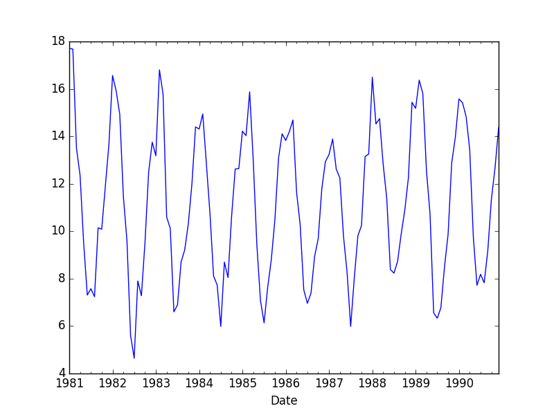
Minimum Monthly Temperature Dataset

We can test the same differencing method on the monthly data and confirm that the seasonally adjusted dataset does indeed remove the yearly cycles.

from pandas import read_csv from matplotlib import pyplot series = read_csv('daily-minimum-temperatures.csv', header=0, index_col=0) resample = series.resample('M') monthly_mean = resample.mean() X = series.values diff = list() months_in_year = 12 for i in range(months_in_year, len(monthly_mean)): value = monthly_mean[i] - monthly_mean[i - months_in_year] diff.append(value) pyplot.plot(diff) pyplot.show()

Running the example creates a new seasonally adjusted monthly minimum temperature dataset, skipping the first year of data in order to create the adjustment. The adjusted dataset is then plotted.

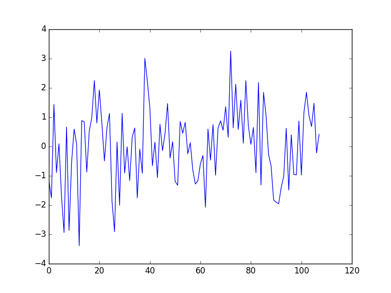
Seasonally Adjusted Minimum Monthly Temperature Dataset

Next, we can use the monthly average minimum temperatures from the same month in the previous year to adjust the daily minimum temperature dataset.

Again, we just skip the first year of data, but the correction using the monthly rather than the daily data may be a more stable approach.

from pandas import read_csv from matplotlib import pyplot series = read_csv('daily-minimum-temperatures.csv', header=0, index_col=0) X = series.values diff = list() days_in_year = 365 for i in range(days_in_year, len(X)): month_str = str(series.index[i].year-1)+'-'+str(series.index[i].month) month_mean_last_year = series[month_str].mean() value = X[i] - month_mean_last_year diff.append(value) pyplot.plot(diff) pyplot.show()

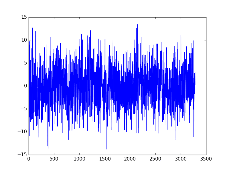
Running the example again creates the seasonally adjusted dataset and plots the results.

This example is robust to daily fluctuations in the previous year and to offset errors creeping in due to February 29 days in leap years.

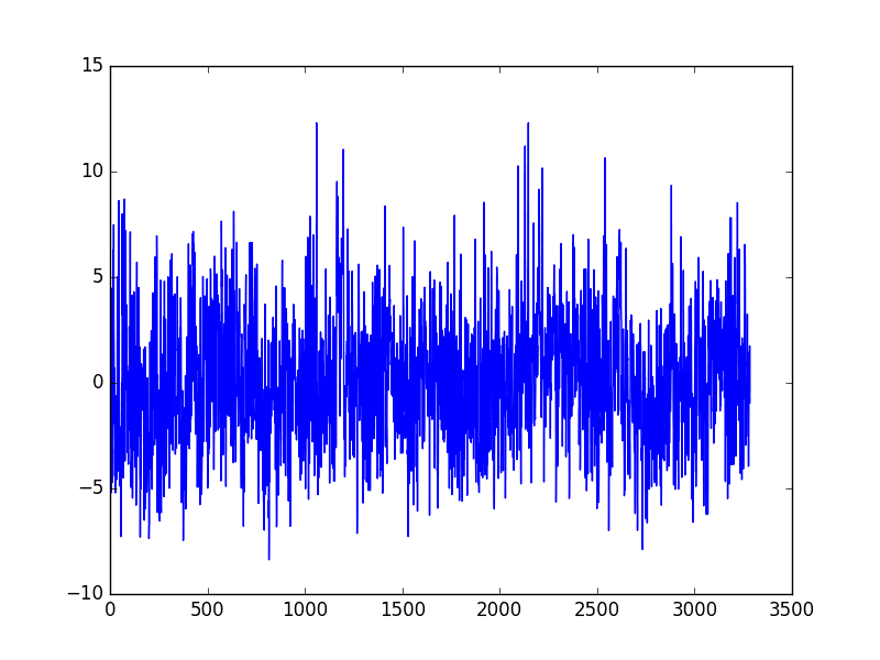
More Stable Seasonally Adjusted Minimum Monthly Temperature Dataset

The edge of calendar months provides a hard boundary that may not make sense for temperature data.

More flexible approaches that take the average from one week either side of the same date in the previous year may again be a better approach.

Additionally, there is likely to be seasonality in temperature data at multiple scales that may be corrected for directly or indirectly, such as:

• Day level.
• Multiple day level, such as a week or weeks.
• Multiple week level, such as a month.
• Multiple month level, such as a quarter or season.

Seasonal Adjustment with Modeling

We can model the seasonal component directly, then subtract it from the observations.

The seasonal component in a given time series is likely a sine wave over a generally fixed period and amplitude. This can be approximated easily using a curve-fitting method.

A dataset can be constructed with the time index of the sine wave as an input, or x-axis, and the observation as the output, or y-axis.

For example:

Time Index, Observation 1, obs1 2, obs2 3, obs3 4, obs4 5, obs5

Once fit, the model can then be used to calculate a seasonal component for any time index.

In the case of the temperature data, the time index would be the day of the year. We can then estimate the seasonal component for the day of the year for any historical observations or any new observations in the future.

The curve can then be used as a new input for modeling with supervised learning algorithms, or subtracted from observations to create a seasonally adjusted series.

Let’s start off by fitting a curve to the Minimum Daily Temperatures dataset. The NumPy library provides the polyfit() function that can be used to fit a polynomial of a chosen order to a dataset.

First, we can create a dataset of time index (day in this case) to observation. We could take a single year of data or all the years. Ideally, we would try both and see which model resulted in a better fit. We could also smooth the observations using a moving average centered on each value. This too may result in a model with a better fit.

Once the dataset is prepared, we can create the fit by calling the polyfit() function passing the x-axis values (integer day of year), y-axis values (temperature observations), and the order of the polynomial. The order controls the number of terms, and in turn the complexity of the curve used to fit the data.

Ideally, we want the simplest curve that describes the seasonality of the dataset. For consistent sine wave-like seasonality, a 4th order or 5th order polynomial will be sufficient.

In this case, I chose an order of 4 by trial and error. The resulting model takes the form:

y = x^4*b1 + x^3*b2 + x^2*b3 + x^1*b4 + b5

Where y is the fit value, x is the time index (day of the year), and b1 to b5 are the coefficients found by the curve-fitting optimization algorithm.

Once fit, we will have a set of coefficients that represent our model. We can then use this model to calculate the curve for one observation, one year of observations, or the entire dataset.

The complete example is listed below.

from pandas import read_csv from matplotlib import pyplot from numpy import polyfit series = read_csv('daily-minimum-temperatures.csv', header=0, index_col=0) # fit polynomial: x^2*b1 + x*b2 + ... + bn X = [i%365 for i in range(0, len(series))] y = series.values degree = 4 coef = polyfit(X, y, degree) print('Coefficients: %s' % coef) # create curve curve = list() for i in range(len(X)): value = coef[-1] for d in range(degree): value += X[i]**(degree-d) * coef[d] curve.append(value) # plot curve over original data pyplot.plot(series.values) pyplot.plot(curve, color='red', linewidth=3) pyplot.show()

Running the example creates the dataset, fits the curve, predicts the value for each day in the dataset, and then plots the resulting seasonal model (red) over the top of the original dataset (blue).

One limitation of this model is that it does not take into account of leap days, adding small offset noise that could easily be corrected with an update to the approach.

For example, we could just remove the two February 29 observations from the dataset when creating the seasonal model.

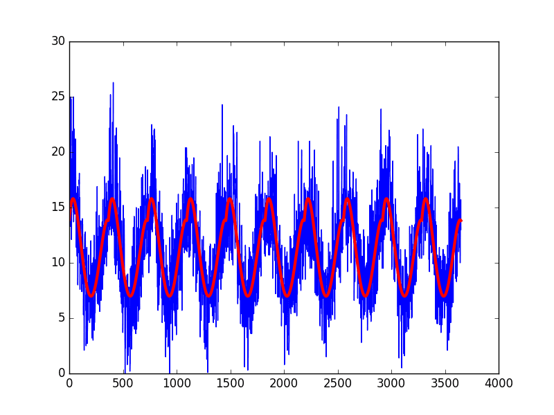
Curve Fit Seasonal Model of Daily Minimum Temperature

The curve appears to be a good fit for the seasonal structure in the dataset.

We can now use this model to create a seasonally adjusted version of the dataset.

The complete example is listed below.

from pandas import read_csv from matplotlib import pyplot from numpy import polyfit series = read_csv('daily-minimum-temperatures.csv', header=0, index_col=0) # fit polynomial: x^2*b1 + x*b2 + ... + bn X = [i%365 for i in range(0, len(series))] y = series.values degree = 4 coef = polyfit(X, y, degree) print('Coefficients: %s' % coef) # create curve curve = list() for i in range(len(X)): value = coef[-1] for d in range(degree): value += X[i]**(degree-d) * coef[d] curve.append(value) # create seasonally adjusted values = series.values diff = list() for i in range(len(values)): value = values[i] - curve[i] diff.append(value) pyplot.plot(diff) pyplot.show()

Running the example subtracts the values predicted by the seasonal model from the original observations. The

The seasonally adjusted dataset is then plotted.

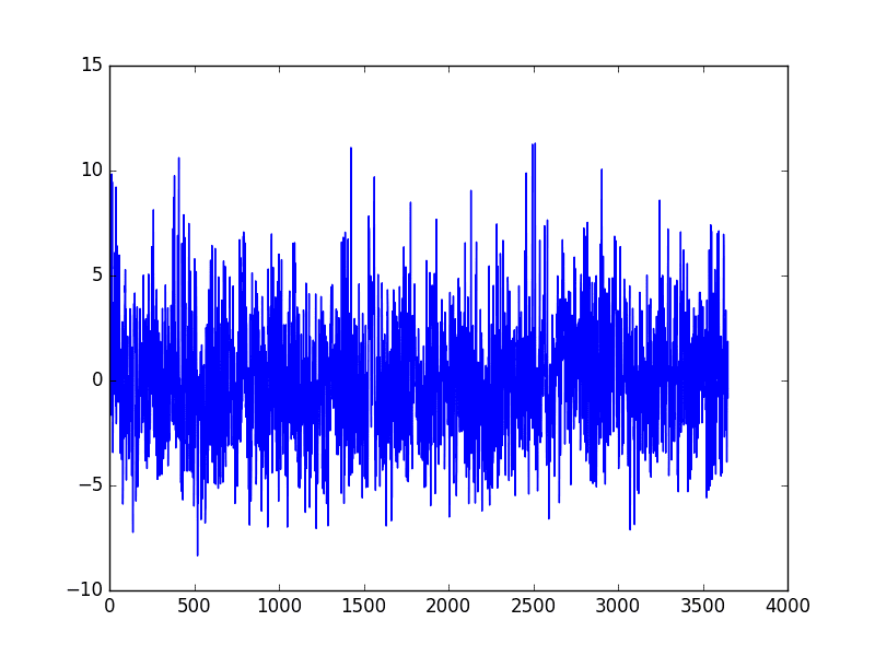
Curve Fit Seasonally Adjusted Daily Minimum Temperature

Summary

In this tutorial, you discovered how to create seasonally adjusted time series datasets in Python.

Specifically, you learned:

• The importance of seasonality in time series and the opportunities for data preparation and feature engineering it provides.
• How to use the difference method to create a seasonally adjusted time series.
• How to model the seasonal component directly and subtract it from observations.

Do you have any questions about deseasonalizing time series, or about this post?
Ask your questions in the comments below and I will do my best to answer.