How to Use Statistical Significance Tests to Interpret Machine Learning Results

 It is good practice to gather a population of results when comparing two different machine learning algorithms or when comparing the same algorithm with different configurations.

Repeating each experimental run 30 or more times gives you a population of results from which you can calculate the mean expected performance, given the stochastic nature of most machine learning algorithms.

If the mean expected performance from two algorithms or configurations are different, how do you know that the difference is significant, and how significant?

Statistical significance tests are an important tool to help to interpret the results from machine learning experiments. Additionally, the findings from these tools can help you better and more confidently present your experimental results and choose the right algorithms and configurations for your predictive modeling problem.

In this tutorial, you will discover how you can investigate and interpret machine learning experimental results using statistical significance tests in Python.

After completing this tutorial, you will know:

• How to apply normality tests to confirm that your data is (or is not) normally distributed.
• How to apply parametric statistical significance tests for normally distributed results.
• How to apply nonparametric statistical significance tests for more complex distributions of results.

  Tutorial Overview

  This tutorial is broken down into 6 parts. They are:

  1. Generate Sample Data
  2. Summary Statistics
  3. Normality Test
  4. Compare Means for Gaussian Results
  5. Compare Means for Gaussian Results with Different Variance
  6. Compare Means for Non-Gaussian Results

  This tutorial assumes Python 2 or 3 and a SciPy environment with NumPy, Pandas, and Matplotlib.

  Generate Sample Data

  The situation is that you have experimental results from two algorithms or two different configurations of the same algorithm.

  Each algorithm has been trialed multiple times on the test dataset and a skill score has been collected. We are left with two populations of skill scores.

  We can simulate this by generating two populations of Gaussian random numbers distributed around slightly different means.

  The code below generates the results from the first algorithm. A total of 1000 results are stored in a file named results1.csv. The results are drawn from a Gaussian distribution with the mean of 50 and the standard deviation of 10.

  from numpy.random import seed from numpy.random import normal from numpy import savetxt # define underlying distribution of results mean = 50 stev = 10 # generate samples from ideal distribution seed(1) results = normal(mean, stev, 1000) # save to ASCII file savetxt('results1.csv', results)

  Below is a snippet of the first 5 rows of data from results1.csv.

  6.624345363663240960e+01 4.388243586349924641e+01 4.471828247736544171e+01 3.927031377843829318e+01 5.865407629324678851e+01 ...

  We can now generate the results for the second algorithm. We will use the same method and draw the results from a slightly different Gaussian distribution (mean of 60 with the same standard deviation). Results are written to results2.csv.

  from numpy.random import seed from numpy.random import normal from numpy import savetxt # define underlying distribution of results mean = 60 stev = 10 # generate samples from ideal distribution seed(1) results = normal(mean, stev, 1000) # save to ASCII file savetxt('results2.csv', results)

  Below is a sample of the first 5 rows from results2.csv.

  7.624345363663240960e+01 5.388243586349924641e+01 5.471828247736544171e+01 4.927031377843829318e+01 6.865407629324678851e+01 ...

  Going forward, we will pretend that we don’t know the underlying distribution of either set of results.

  I chose populations of 1000 results per experiment arbitrarily. It is more realistic to use populations of 30 or 100 results to achieve a suitably good estimate (e.g. low standard error).

  Don’t worry if your results are not Gaussian; we will look at how the methods break down for non-Gaussian data and what alternate methods to use instead.

  Summary Statistics

  The first step after collecting results is to review some summary statistics and learn more about the distribution of the data.

  This includes reviewing summary statistics and plots of the data.

  Below is a complete code listing to review some summary statistics for the two sets of results.

  from pandas import DataFrame from pandas import read_csv from matplotlib import pyplot # load results file results = DataFrame() results['A'] = read_csv('results1.csv', header=None).values[:, 0] results['B'] = read_csv('results2.csv', header=None).values[:, 0] # descriptive stats print(results.describe()) # box and whisker plot results.boxplot() pyplot.show() # histogram results.hist() pyplot.show()

  The example loads both sets of results and starts off by printing summary statistics. Data in results1.csv is called “A” and data in results2.csv is called “B” for brevity.

  We will assume that the data represents an error score on a test dataset and that minimizing the score is the goal.

  We can see that on average A (50.388125) was better than B (60.388125). We can also see the same story in the median (50th percentile). Looking at the standard deviations, we can also see that it appears both distributions have a similar (identical) spread.

  A            B count  1000.000000  1000.000000 mean     50.388125    60.388125 std       9.814950     9.814950 min      19.462356    29.462356 25%      43.998396    53.998396 50%      50.412926    60.412926 75%      57.039989    67.039989 max      89.586027    99.586027

  Next, a box and whisker plot is created comparing both sets of results. The box captures the middle 50% of the data, outliers are shown as dots and the green line shows the median. We can see the data indeed has a similar spread from both distributions and appears to be symmetrical around the median.

  The results for A look better than B.

  

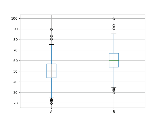
  Box and Whisker Plots of Both Sets of Results

  Finally, histograms of both sets of results are plotted.

  The plots strongly suggest that both sets of results are drawn from a Gaussian distribution.

  

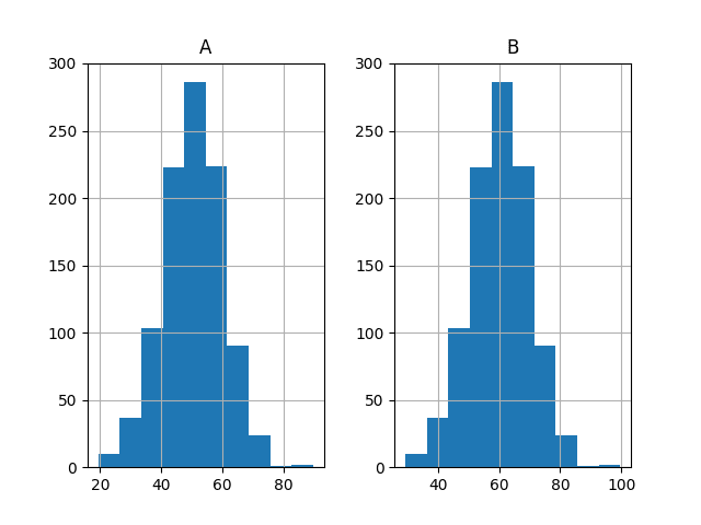
  Histogram Plots of Both Sets of Results

  Normality Test

  Data drawn from a Gaussian distribution can be easier to work with as there are many tools and techniques specifically designed for this case.

  We can use a statistical test to confirm that the results drawn from both distributions are Gaussian (also called the normal distribution).

  In SciPy, this is the normaltest() function.

  From the documentation, the test is described as:

  Tests whether a sample differs from a normal distribution.

  The null hypothesis of the test (H0), or the default expectation, is that the statistic describes a normal distribution.

  We fail to reject this hypothesis if the p-value is greater than 0.05. We reject this hypothesis if the p-value <= 0.05. In this case, we would believe the distribution is not normal with 95% confidence.

  The code below loads results1.csv and determines whether it is likely that the data is Gaussian.

  from pandas import read_csv from scipy.stats import normaltest from matplotlib import pyplot result1 = read_csv('results1.csv', header=None) value, p = normaltest(result1.values[:,0]) print(value, p) if p >= 0.05: print('It is likely that result1 is normal') else: print('It is unlikely that result1 is normal')

  Running the example first prints the calculated statistic and the p-value that the statistic was calculated from a Gaussian distribution.

  We can see that it is very likely that results1.csv is Gaussian.

  2.99013078116 0.224233941463 It is likely that result1 is normal

  We can repeat this same test with data from results2.csv.

  The complete code listing is provided below.

  from pandas import read_csv from scipy.stats import normaltest from matplotlib import pyplot result2 = read_csv('results2.csv', header=None) value, p = normaltest(result2.values[:,0]) print(value, p) if p >= 0.05: print('It is likely that result2 is normal') else: print('It is unlikely that result2 is normal')

  Running the example provides the same statistic p-value and outcome.

  Both sets of results are Gaussian.

  2.99013078116 0.224233941463 It is likely that result2 is normal

  Compare Means for Gaussian Results

  Both sets of results are Gaussian and have the same variance; this means we can use the Student t-test to see if the difference between the means of the two distributions is statistically significant or not.

  In SciPy, we can use the ttest_ind() function.

  The test is described as:

  Calculates the T-test for the means of two independent samples of scores.

  The null hypothesis of the test (H0) or the default expectation is that both samples were drawn from the same population. If we fail to reject this hypothesis, it means that there is no significant difference between the means.

  If we get a p-value of <= 0.05, it means that we can reject the null hypothesis and that the means are significantly different with a 95% confidence. That means for 95 similar samples out of 100, the means would be significantly different, and not so in 5 out of 100 cases.

  An important assumption of this statistical test, besides the data being Gaussian, is that both distributions have the same variance. We know this to be the case from reviewing the descriptive statistics in a previous step.

  The complete code listing is provided below.

  from pandas import read_csv from scipy.stats import ttest_ind from matplotlib import pyplot # load results1 result1 = read_csv('results1.csv', header=None) values1 = result1.values[:,0] # load results2 result2 = read_csv('results2.csv', header=None) values2 = result2.values[:,0] # calculate the significance value, pvalue = ttest_ind(values1, values2, equal_var=True) print(value, pvalue) if pvalue > 0.05: print('Samples are likely drawn from the same distributions (fail to reject H0)') else: print('Samples are likely drawn from different distributions (reject H0)')

  Running the example prints the statistic and the p-value. We can see that the p-value is much lower than 0.05.

  In fact, it is so small that we have a near certainty that the difference between the means is statistically significant.

  -22.7822655028 2.5159901708e-102 Samples are likely drawn from different distributions (reject H0)

  Compare Means for Gaussian Results with Different Variance

  What if the means were the same for the two sets of results, but the variance was different?

  We would not be able to use the Student t-test as is. In fact, we would have to use a modified version of the test called Welch’s t-test.

  In SciPy, this is the same ttest_ind() function, but we must set the “equal_var” argument to “False” to indicate the variances are not equal.

  We can demonstrate this with an example where we generate two sets of results with means that are very similar (50 vs 51) and very different standard deviations (1 vs 10). We will generate 100 samples.

  from numpy.random import seed from numpy.random import normal from scipy.stats import ttest_ind # generate results seed(1) n = 100 values1 = normal(50, 1, n) values2 = normal(51, 10, n) # calculate the significance value, pvalue = ttest_ind(values1, values2, equal_var=False) print(value, pvalue) if pvalue > 0.05: print('Samples are likely drawn from the same distributions (fail to reject H0)') else: print('Samples are likely drawn from different distributions (reject H0)')

  Running the example prints the test statistic and the p-value.

  We can see that there is good evidence (nearly 99%) that the samples were drawn from different distributions, that the means are significantly different.

  -2.62233137406 0.0100871483783 Samples are likely drawn from different distributions (reject H0)

  The closer the distributions are, the larger the sample that is required to tell them apart.

  We can demonstrate this by calculating the statistical test on different sized sub-samples of each set of results and plotting the p-values against the sample size.

  We would expect the p-value to get smaller with the increase sample size. We can also draw a line at the 95% level (0.05) and show at what point the sample size is large enough to indicate these two populations are significantly different.

  from numpy.random import seed from numpy.random import normal from scipy.stats import ttest_ind from matplotlib import pyplot # generate results seed(1) n = 100 values1 = normal(50, 1, n) values2 = normal(51, 10, n) # calculate p-values for different subsets of results pvalues = list() for i in range(1, n+1): value, p = ttest_ind(values1[0:i], values2[0:i], equal_var=False) pvalues.append(p) # plot p-values vs number of results in sample pyplot.plot(pvalues) # draw line at 95%, below which we reject H0 pyplot.plot([0.05 for x in range(len(pvalues))], color='red') pyplot.show()

  Running the example creates a line plot of p-value vs sample size.

  We can see that for these two sets of results, the sample size must be about 90 before we have a 95% confidence that the means are significantly different (where the blue line intersects the red line).

  

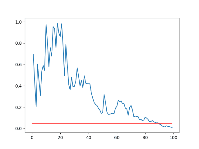
  Line Plot of p-value vs Sample Sizes

  Compare Means for Non-Gaussian Results

  We cannot use the Student t-test or the Welch’s t-test if our data is not Gaussian.

  An alternative statistical significance test we can use for non-Gaussian data is called the Kolmogorov-Smirnov test.

  In SciPy, this is called the ks_2samp() function.

  In the documentation, this test is described as:

  This is a two-sided test for the null hypothesis that 2 independent samples are drawn from the same continuous distribution.

  This test can be used on Gaussian data, but will have less statistical power and may require large samples.

  We can demonstrate the calculation of statistical significance on two sets of results with non-Gaussian distributions. We can generate two sets of results with overlapping uniform distributions (50 to 60 and 55 to 65). These sets of results will have different mean values of about 55 and 60 respectively.

  The code below generates the two sets of 100 results and uses the Kolmogorov-Smirnov test to demonstrate that the difference between the population means is statistically significant.

  from numpy.random import seed from numpy.random import randint from scipy.stats import ks_2samp # generate results seed(1) n = 100 values1 = randint(50, 60, n) values2 = randint(55, 65, n) # calculate the significance value, pvalue = ks_2samp(values1, values2) print(value, pvalue) if pvalue > 0.05: print('Samples are likely drawn from the same distributions (fail to reject H0)') else: print('Samples are likely drawn from different distributions (reject H0)')

  Running the example prints the statistic and the p-value.

  The p-value is very small, suggesting a near certainty that the difference between the two populations is significant.

  0.47 2.16825856737e-10 Samples are likely drawn from different distributions (reject H0)

  Further Reading

  This section lists some articles and resources to dive deeper into the area of statistical significance testing for applied machine learning.

  • Normality test on Wikipedia
  • Student’s t-test on Wikipedia
  • Welch’s t-test on Wikipedia
  • Kolmogorov–Smirnov test on Wikipedia

  Summary

  In this tutorial, you discovered how you can use statistical significance tests to interpret machine learning results.

  You can use these tests to help you confidently choose one machine learning algorithm over another or one set of configuration parameters over another for the same algorithm.

  You learned:

  • How to use normality tests to check if your experimental results are Gaussian or not.
  • How to use statistical tests to check if the difference between mean results is significant for Gaussian data with the same and different variance.
  • How to use statistical tests to check if the difference between mean results is significant for non-Gaussian data.

  Do you have any questions about this post or statistical significance tests?
  Ask your questions in the comments below and I will do my best to answer.