Dropout with LSTM Networks for Time Series Forecasting

 Long Short-Term Memory (LSTM) models are a type of recurrent neural network capable of learning sequences of observations.

This may make them a network well suited to time series forecasting.

An issue with LSTMs is that they can easily overfit training data, reducing their predictive skill.

Dropout is a regularization method where input and recurrent connections to LSTM units are probabilistically excluded from activation and weight updates while training a network. This has the effect of reducing overfitting and improving model performance.

In this tutorial, you will discover how to use dropout with LSTM networks and design experiments to test for its effectiveness for time series forecasting.

After completing this tutorial, you will know:

• How to design a robust test harness for evaluating LSTM networks for time series forecasting.
• How to design, execute, and interpret the results from using input weight dropout with LSTMs.
• How to design, execute, and interpret the results from using recurrent weight dropout with LSTMs.

  Tutorial Overview

  This tutorial is broken down into 5 parts. They are:

  1. Shampoo Sales Dataset
  2. Experimental Test Harness
  3. Input Dropout
  4. Recurrent Dropout
  5. Review of Results

  Environment

  This tutorial assumes you have a Python SciPy environment installed. You can use either Python 2 or 3 with this example.

  This tutorial assumes you have Keras v2.0 or higher installed with either the TensorFlow or Theano backend.

  This tutorial also assumes you have scikit-learn, Pandas, NumPy, and Matplotlib installed.

  Next, let’s take a look at a standard time series forecasting problem that we can use as context for this experiment.

  If you need help setting up your Python environment, see this post:

  • How to Setup a Python Environment for Machine Learning and Deep Learning with Anaconda

  Need help with Deep Learning for Time Series?

  Take my free 7-day email crash course now (with sample code).

  Click to sign-up and also get a free PDF Ebook version of the course.

  Shampoo Sales Dataset

  This dataset describes the monthly number of sales of shampoo over a 3-year period.

  The units are a sales count and there are 36 observations. The original dataset is credited to Makridakis, Wheelwright, and Hyndman (1998).

  • Download the dataset.

  The example below loads and creates a plot of the loaded dataset.

  # load and plot dataset from pandas import read_csv from pandas import datetime from matplotlib import pyplot # load dataset def parser(x): return datetime.strptime('190'+x, '%Y-%m') series = read_csv('shampoo-sales.csv', header=0, parse_dates=[0], index_col=0, squeeze=True, date_parser=parser) # summarize first few rows print(series.head()) # line plot series.plot() pyplot.show()

  Running the example loads the dataset as a Pandas Series and prints the first 5 rows.

  Month 1901-01-01 266.0 1901-02-01 145.9 1901-03-01 183.1 1901-04-01 119.3 1901-05-01 180.3 Name: Sales, dtype: float64

  A line plot of the series is then created showing a clear increasing trend.

  

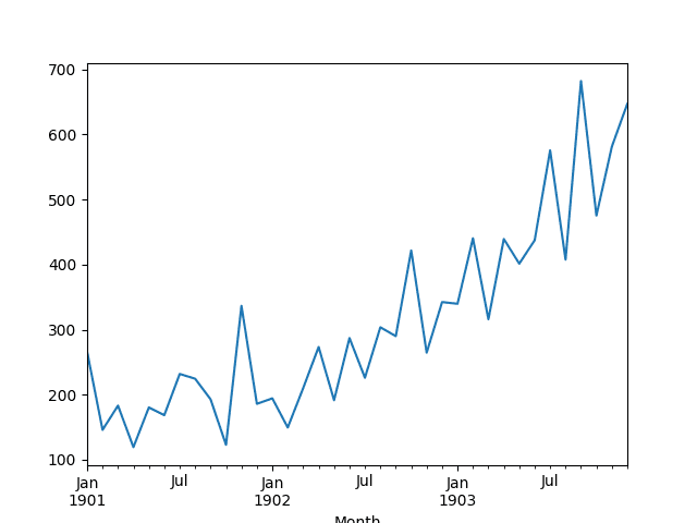
  Line Plot of Shampoo Sales Dataset

  Next, we will take a look at the model configuration and test harness used in the experiment.

  Experimental Test Harness

  This section describes the test harness used in this tutorial.

  Data Split

  We will split the Shampoo Sales dataset into two parts: a training and a test set.

  The first two years of data will be taken for the training dataset and the remaining one year of data will be used for the test set.

  Models will be developed using the training dataset and will make predictions on the test dataset.

  The persistence forecast (naive forecast) on the test dataset achieves an error of 136.761 monthly shampoo sales. This provides a lower acceptable bound of performance on the test set.

  Model Evaluation

  A rolling-forecast scenario will be used, also called walk-forward model validation.

  Each time step of the test dataset will be walked one at a time. A model will be used to make a forecast for the time step, then the actual expected value from the test set will be taken and made available to the model for the forecast on the next time step.

  This mimics a real-world scenario where new Shampoo Sales observations would be available each month and used in the forecasting of the following month.

  This will be simulated by the structure of the train and test datasets.

  All forecasts on the test dataset will be collected and an error score calculated to summarize the skill of the model. The root mean squared error (RMSE) will be used as it punishes large errors and results in a score that is in the same units as the forecast data, namely monthly shampoo sales.

  Data Preparation

  Before we can fit a model to the dataset, we must transform the data.

  The following three data transforms are performed on the dataset prior to fitting a model and making a forecast.

  1. Transform the time series data so that it is stationary. Specifically, a lag=1 differencing to remove the increasing trend in the data.
  2. Transform the time series into a supervised learning problem. Specifically, the organization of data into input and output patterns where the observation at the previous time step is used as an input to forecast the observation at the current time step
  3. Transform the observations to have a specific scale. Specifically, to rescale the data to values between -1 and 1.

  These transforms are inverted on forecasts to return them into their original scale before calculating and error score.

  LSTM Model

  We will use a base stateful LSTM model with 1 neuron fit for 1000 epochs.

  A batch size of 1 is required as we will be using walk-forward validation and making one-step forecasts for each of the final 12 months of test data.

  A batch size of 1 means that the model will be fit using online training (as opposed to batch training or mini-batch training). As a result, it is expected that the model fit will have some variance.

  Ideally, more training epochs would be used (such as 1500), but this was truncated to 1000 to keep run times reasonable.

  The model will be fit using the efficient ADAM optimization algorithm and the mean squared error loss function.

  Experimental Runs

  Each experimental scenario will be run 30 times and the RMSE score on the test set will be recorded from the end each run.

  Let’s dive into the experiments.

  Baseline LSTM Model

  Let’s start off with the baseline LSTM model.

  The baseline LSTM model for this problem has the following configuration:

  • Lag inputs: 1
  • Epochs: 1000
  • Units in LSTM hidden layer: 3
  • Batch Size: 4
  • Repeats: 3

  The complete code listing is provided below.

  This code listing will be used as the basis for all following experiments, with only the changes to this code listing provided in subsequent sections.

  from pandas import DataFrame from pandas import Series from pandas import concat from pandas import read_csv from pandas import datetime from sklearn.metrics import mean_squared_error from sklearn.preprocessing import MinMaxScaler from keras.models import Sequential from keras.layers import Dense from keras.layers import LSTM from math import sqrt import matplotlib # be able to save images on server matplotlib.use('Agg') from matplotlib import pyplot import numpy   # date-time parsing function for loading the dataset def parser(x): return datetime.strptime('190'+x, '%Y-%m')   # frame a sequence as a supervised learning problem def timeseries_to_supervised(data, lag=1): df = DataFrame(data) columns = [df.shift(i) for i in range(1, lag+1)] columns.append(df) df = concat(columns, axis=1) return df   # create a differenced series def difference(dataset, interval=1): diff = list() for i in range(interval, len(dataset)): value = dataset[i] - dataset[i - interval] diff.append(value) return Series(diff)   # invert differenced value def inverse_difference(history, yhat, interval=1): return yhat + history[-interval]   # scale train and test data to [-1, 1] def scale(train, test): # fit scaler scaler = MinMaxScaler(feature_range=(-1, 1)) scaler = scaler.fit(train) # transform train train = train.reshape(train.shape[0], train.shape[1]) train_scaled = scaler.transform(train) # transform test test = test.reshape(test.shape[0], test.shape[1]) test_scaled = scaler.transform(test) return scaler, train_scaled, test_scaled   # inverse scaling for a forecasted value def invert_scale(scaler, X, yhat): new_row = [x for x in X] + [yhat] array = numpy.array(new_row) array = array.reshape(1, len(array)) inverted = scaler.inverse_transform(array) return inverted[0, -1]   # fit an LSTM network to training data def fit_lstm(train, n_batch, nb_epoch, n_neurons): X, y = train[:, 0:-1], train[:, -1] X = X.reshape(X.shape[0], 1, X.shape[1]) model = Sequential() model.add(LSTM(n_neurons, batch_input_shape=(n_batch, X.shape[1], X.shape[2]), stateful=True)) model.add(Dense(1)) model.compile(loss='mean_squared_error', optimizer='adam') for i in range(nb_epoch): model.fit(X, y, epochs=1, batch_size=n_batch, verbose=0, shuffle=False) model.reset_states() return model   # run a repeated experiment def experiment(series, n_lag, n_repeats, n_epochs, n_batch, n_neurons): # transform data to be stationary raw_values = series.values diff_values = difference(raw_values, 1) # transform data to be supervised learning supervised = timeseries_to_supervised(diff_values, n_lag) supervised_values = supervised.values[n_lag:,:] # split data into train and test-sets train, test = supervised_values[0:-12], supervised_values[-12:] # transform the scale of the data scaler, train_scaled, test_scaled = scale(train, test) # run experiment error_scores = list() for r in range(n_repeats): # fit the model train_trimmed = train_scaled[2:, :] lstm_model = fit_lstm(train_trimmed, n_batch, n_epochs, n_neurons) # forecast test dataset test_reshaped = test_scaled[:,0:-1] test_reshaped = test_reshaped.reshape(len(test_reshaped), 1, 1) output = lstm_model.predict(test_reshaped, batch_size=n_batch) predictions = list() for i in range(len(output)): yhat = output[i,0] X = test_scaled[i, 0:-1] # invert scaling yhat = invert_scale(scaler, X, yhat) # invert differencing yhat = inverse_difference(raw_values, yhat, len(test_scaled)+1-i) # store forecast predictions.append(yhat) # report performance rmse = sqrt(mean_squared_error(raw_values[-12:], predictions)) print('%d) Test RMSE: %.3f' % (r+1, rmse)) error_scores.append(rmse) return error_scores   # configure the experiment def run(): # load dataset series = read_csv('shampoo-sales.csv', header=0, parse_dates=[0], index_col=0, squeeze=True, date_parser=parser) # configure the experiment n_lag = 1 n_repeats = 30 n_epochs = 1000 n_batch = 4 n_neurons = 3 # run the experiment results = DataFrame() results['results'] = experiment(series, n_lag, n_repeats, n_epochs, n_batch, n_neurons) # summarize results print(results.describe()) # save boxplot results.boxplot() pyplot.savefig('experiment_baseline.png')   # entry point run()

  Running the experiment prints summary statistics for the test RMSE for all repeats.

  Note: Your results may vary given the stochastic nature of the algorithm or evaluation procedure, or differences in numerical precision. Consider running the example a few times and compare the average outcome.

  We can see that on average this model configuration achieved a test RMSE of about 92 monthly shampoo sales with a standard deviation of 5.

  results count   30.000000 mean    92.842537 std      5.748456 min     81.205979 25%     89.514367 50%     92.030003 75%     96.926145 max    105.247117

  A box and whisker plot is also created from the distribution of test RMSE results and saved to a file.

  The plot provides a clear depiction of the spread of the results, highlighting the middle 50% of values (the box) and the median (green line).

  

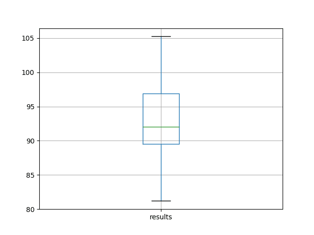
  Box and Whisker Plot of Baseline Performance on the Shampoo Sales Dataset

  Another angle to consider with a network configuration is how it behaves over time as the model is being fit.

  We can evaluate the model on the training and test datasets after each training epoch to get an idea as to if the configuration is overfitting or underfitting the problem.

  We will use this diagnostic approach on the top result from each set of experiments. A total of 10 repeats of the configuration will be run and the train and test RMSE scores after each training epoch plotted on a line plot.

  In this case, we will use this diagnostic on the LSTM fit for 1000 epochs.

  The complete diagnostic code listing is provided below.

  As with the previous code listing, the code below will be used as the basis for all diagnostics in this tutorial and only the changes to this listing will be provided in subsequent sections.

  from pandas import DataFrame from pandas import Series from pandas import concat from pandas import read_csv from pandas import datetime from sklearn.metrics import mean_squared_error from sklearn.preprocessing import MinMaxScaler from keras.models import Sequential from keras.layers import Dense from keras.layers import LSTM from math import sqrt import matplotlib # be able to save images on server matplotlib.use('Agg') from matplotlib import pyplot import numpy   # date-time parsing function for loading the dataset def parser(x): return datetime.strptime('190'+x, '%Y-%m')   # frame a sequence as a supervised learning problem def timeseries_to_supervised(data, lag=1): df = DataFrame(data) columns = [df.shift(i) for i in range(1, lag+1)] columns.append(df) df = concat(columns, axis=1) return df   # create a differenced series def difference(dataset, interval=1): diff = list() for i in range(interval, len(dataset)): value = dataset[i] - dataset[i - interval] diff.append(value) return Series(diff)   # scale train and test data to [-1, 1] def scale(train, test): # fit scaler scaler = MinMaxScaler(feature_range=(-1, 1)) scaler = scaler.fit(train) # transform train train = train.reshape(train.shape[0], train.shape[1]) train_scaled = scaler.transform(train) # transform test test = test.reshape(test.shape[0], test.shape[1]) test_scaled = scaler.transform(test) return scaler, train_scaled, test_scaled   # inverse scaling for a forecasted value def invert_scale(scaler, X, yhat): new_row = [x for x in X] + [yhat] array = numpy.array(new_row) array = array.reshape(1, len(array)) inverted = scaler.inverse_transform(array) return inverted[0, -1]   # evaluate the model on a dataset, returns RMSE in transformed units def evaluate(model, raw_data, scaled_dataset, scaler, offset, batch_size): # separate X, y = scaled_dataset[:,0:-1], scaled_dataset[:,-1] # reshape reshaped = X.reshape(len(X), 1, 1) # forecast dataset output = model.predict(reshaped, batch_size=batch_size) # invert data transforms on forecast predictions = list() for i in range(len(output)): yhat = output[i,0] # invert scaling yhat = invert_scale(scaler, X[i], yhat) # invert differencing yhat = yhat + raw_data[i] # store forecast predictions.append(yhat) # report performance rmse = sqrt(mean_squared_error(raw_data[1:], predictions)) # reset model state model.reset_states() return rmse   # fit an LSTM network to training data def fit_lstm(train, test, raw, scaler, batch_size, nb_epoch, neurons): X, y = train[:, 0:-1], train[:, -1] X = X.reshape(X.shape[0], 1, X.shape[1]) # prepare model model = Sequential() model.add(LSTM(neurons, batch_input_shape=(batch_size, X.shape[1], X.shape[2]), stateful=True)) model.add(Dense(1)) model.compile(loss='mean_squared_error', optimizer='adam') # fit model train_rmse, test_rmse = list(), list() for i in range(nb_epoch): model.fit(X, y, epochs=1, batch_size=batch_size, verbose=0, shuffle=False) model.reset_states() # evaluate model on train data raw_train = raw[-(len(train)+len(test)+1):-len(test)] train_rmse.append(evaluate(model, raw_train, train, scaler, 0, batch_size)) # evaluate model on test data raw_test = raw[-(len(test)+1):] test_rmse.append(evaluate(model, raw_test, test, scaler, 0, batch_size)) history = DataFrame() history['train'], history['test'] = train_rmse, test_rmse return history   # run diagnostic experiments def run(): # config n_lag = 1 n_repeats = 10 n_epochs = 1000 n_batch = 4 n_neurons = 3 # load dataset series = read_csv('shampoo-sales.csv', header=0, parse_dates=[0], index_col=0, squeeze=True, date_parser=parser) # transform data to be stationary raw_values = series.values diff_values = difference(raw_values, 1) # transform data to be supervised learning supervised = timeseries_to_supervised(diff_values, n_lag) supervised_values = supervised.values[n_lag:,:] # split data into train and test-sets train, test = supervised_values[0:-12], supervised_values[-12:] # transform the scale of the data scaler, train_scaled, test_scaled = scale(train, test) # fit and evaluate model train_trimmed = train_scaled[2:, :] # run diagnostic tests for i in range(n_repeats): history = fit_lstm(train_trimmed, test_scaled, raw_values, scaler, n_batch, n_epochs, n_neurons) pyplot.plot(history['train'], color='blue') pyplot.plot(history['test'], color='orange') print('%d) TrainRMSE=%f, TestRMSE=%f' % (i+1, history['train'].iloc[-1], history['test'].iloc[-1])) pyplot.savefig('diagnostic_baseline.png')   # entry point run()

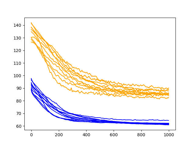
  Running the diagnostic prints the final train and test RMSE for each run. More interesting is the final line plot created.

  The line plot shows the train RMSE (blue) and test RMSE (orange) after each training epoch.

  Note: Your results may vary given the stochastic nature of the algorithm or evaluation procedure, or differences in numerical precision. Consider running the example a few times and compare the average outcome.

  In this case, the diagnostic plot shows a steady decrease in train and test RMSE to about 400-500 epochs, after which time it appears some overfitting may be occurring. This is signified by a continued decrease in train RMSE and an increase in test RMSE.

  

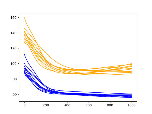
  Diagnostic Line Plot of the Baseline Model on the Shampoo Sales Daset

  Input Dropout

  Dropout can be applied to the input connection within the LSTM nodes.

  A dropout on the input means that for a given probability, the data on the input connection to each LSTM block will be excluded from node activation and weight updates.

  In Keras, this is specified with a dropout argument when creating an LSTM layer. The dropout value is a percentage between 0 (no dropout) and 1 (no connection).

  In this experiment, we will compare no dropout to input dropout rates of 20%, 40% and 60%.

  Below lists the updated fit_lstm(), experiment(), and run() functions for using input dropout with LSTMs.

  # fit an LSTM network to training data def fit_lstm(train, n_batch, nb_epoch, n_neurons, dropout): X, y = train[:, 0:-1], train[:, -1] X = X.reshape(X.shape[0], 1, X.shape[1]) model = Sequential() model.add(LSTM(n_neurons, batch_input_shape=(n_batch, X.shape[1], X.shape[2]), stateful=True, dropout=dropout)) model.add(Dense(1)) model.compile(loss='mean_squared_error', optimizer='adam') for i in range(nb_epoch): model.fit(X, y, epochs=1, batch_size=n_batch, verbose=0, shuffle=False) model.reset_states() return model   # run a repeated experiment def experiment(series, n_lag, n_repeats, n_epochs, n_batch, n_neurons, dropout): # transform data to be stationary raw_values = series.values diff_values = difference(raw_values, 1) # transform data to be supervised learning supervised = timeseries_to_supervised(diff_values, n_lag) supervised_values = supervised.values[n_lag:,:] # split data into train and test-sets train, test = supervised_values[0:-12], supervised_values[-12:] # transform the scale of the data scaler, train_scaled, test_scaled = scale(train, test) # run experiment error_scores = list() for r in range(n_repeats): # fit the model train_trimmed = train_scaled[2:, :] lstm_model = fit_lstm(train_trimmed, n_batch, n_epochs, n_neurons, dropout) # forecast test dataset test_reshaped = test_scaled[:,0:-1] test_reshaped = test_reshaped.reshape(len(test_reshaped), 1, 1) output = lstm_model.predict(test_reshaped, batch_size=n_batch) predictions = list() for i in range(len(output)): yhat = output[i,0] X = test_scaled[i, 0:-1] # invert scaling yhat = invert_scale(scaler, X, yhat) # invert differencing yhat = inverse_difference(raw_values, yhat, len(test_scaled)+1-i) # store forecast predictions.append(yhat) # report performance rmse = sqrt(mean_squared_error(raw_values[-12:], predictions)) print('%d) Test RMSE: %.3f' % (r+1, rmse)) error_scores.append(rmse) return error_scores   # configure the experiment def run(): # load dataset series = read_csv('shampoo-sales.csv', header=0, parse_dates=[0], index_col=0, squeeze=True, date_parser=parser) # configure the experiment n_lag = 1 n_repeats = 30 n_epochs = 1000 n_batch = 4 n_neurons = 3 n_dropout = [0.0, 0.2, 0.4, 0.6] # run the experiment results = DataFrame() for dropout in n_dropout: results[str(dropout)] = experiment(series, n_lag, n_repeats, n_epochs, n_batch, n_neurons, dropout) # summarize results print(results.describe()) # save boxplot results.boxplot() pyplot.savefig('experiment_dropout_input.png')

  Running this experiment prints descriptives statistics for each evaluated configuration.

  Note: Your results may vary given the stochastic nature of the algorithm or evaluation procedure, or differences in numerical precision. Consider running the example a few times and compare the average outcome.

  The results suggest that on average an input dropout of 40% results in better performance, but the difference between the average result for a dropout of 20%, 40%, and 60% is very minor. All seemed to outperform no dropout.

  0.0         0.2        0.4        0.6 count   30.000000   30.000000  30.000000  30.000000 mean    97.578280   89.448450  88.957421  89.810789 std      7.927639    5.807239   4.070037   3.467317 min     84.749785   81.315336  80.662878  84.300135 25%     92.520968   84.712064  85.885858  87.766818 50%     97.324110   88.109654  88.790068  89.585945 75%    101.258252   93.642621  91.515127  91.109452 max    123.578235  104.528209  96.687333  99.660331

  A box and whisker plot is also created to compare the distributions of results for each configuration.

  The plot shows the spread of results decreasing with the increase of input dropout. The plot also suggests that the input dropout of 20% may have a slightly lower median test RMSE.

  The results do encourage the use of some input dropout for the chosen LSTM configuration, perhaps set to 40%.

  

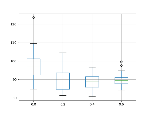
  Box and Whisker Plot of Input Dropout Performance on the Shampoo Sales Dataset

  We can review how input dropout of 40% affects the dynamics of the model while being fit to the training data.

  The code below summarizes the updates to the fit_lstm() and run() functions compared to the baseline version of the diagnostic script.

  # fit an LSTM network to training data def fit_lstm(train, test, raw, scaler, batch_size, nb_epoch, neurons, dropout): X, y = train[:, 0:-1], train[:, -1] X = X.reshape(X.shape[0], 1, X.shape[1]) # prepare model model = Sequential() model.add(LSTM(neurons, batch_input_shape=(batch_size, X.shape[1], X.shape[2]), stateful=True, dropout=dropout)) model.add(Dense(1)) model.compile(loss='mean_squared_error', optimizer='adam') # fit model train_rmse, test_rmse = list(), list() for i in range(nb_epoch): model.fit(X, y, epochs=1, batch_size=batch_size, verbose=0, shuffle=False) model.reset_states() # evaluate model on train data raw_train = raw[-(len(train)+len(test)+1):-len(test)] train_rmse.append(evaluate(model, raw_train, train, scaler, 0, batch_size)) # evaluate model on test data raw_test = raw[-(len(test)+1):] test_rmse.append(evaluate(model, raw_test, test, scaler, 0, batch_size)) history = DataFrame() history['train'], history['test'] = train_rmse, test_rmse return history   # run diagnostic experiments def run(): # config n_lag = 1 n_repeats = 10 n_epochs = 1000 n_batch = 4 n_neurons = 3 dropout = 0.4 # load dataset series = read_csv('shampoo-sales.csv', header=0, parse_dates=[0], index_col=0, squeeze=True, date_parser=parser) # transform data to be stationary raw_values = series.values diff_values = difference(raw_values, 1) # transform data to be supervised learning supervised = timeseries_to_supervised(diff_values, n_lag) supervised_values = supervised.values[n_lag:,:] # split data into train and test-sets train, test = supervised_values[0:-12], supervised_values[-12:] # transform the scale of the data scaler, train_scaled, test_scaled = scale(train, test) # fit and evaluate model train_trimmed = train_scaled[2:, :] # run diagnostic tests for i in range(n_repeats): history = fit_lstm(train_trimmed, test_scaled, raw_values, scaler, n_batch, n_epochs, n_neurons, dropout) pyplot.plot(history['train'], color='blue') pyplot.plot(history['test'], color='orange') print('%d) TrainRMSE=%f, TestRMSE=%f' % (i+1, history['train'].iloc[-1], history['test'].iloc[-1])) pyplot.savefig('diagnostic_dropout_input.png')

  Running the updated diagnostic creates a plot of the train and test RMSE performance of the model with input dropout after each training epoch.

  The results show a clear addition of bumps to the train and test RMSE traces, which is more pronounced on the test RMSE scores.

  We can also see that the symptoms of overfitting have been addressed with test RMSE continuing to go down over the entire 1000 epochs, perhaps suggesting the need for additional training epochs to capitalize on the behavior.

  

  Diagnostic Line Plot of Input Dropout Performance on the Shampoo Sales Dataset

  Recurrent Dropout

  Dropout can also be applied to the recurrent input signal on the LSTM units.

  In Keras, this is achieved by setting the recurrent_dropout argument when defining a LSTM layer.

  In this experiment, we will compare no dropout to the recurrent dropout rates of 20%, 40%, and 60%.

  Below lists the updated fit_lstm(), experiment(), and run() functions for using input dropout with LSTMs.

  # fit an LSTM network to training data def fit_lstm(train, n_batch, nb_epoch, n_neurons, dropout): X, y = train[:, 0:-1], train[:, -1] X = X.reshape(X.shape[0], 1, X.shape[1]) model = Sequential() model.add(LSTM(n_neurons, batch_input_shape=(n_batch, X.shape[1], X.shape[2]), stateful=True, recurrent_dropout=dropout)) model.add(Dense(1)) model.compile(loss='mean_squared_error', optimizer='adam') for i in range(nb_epoch): model.fit(X, y, epochs=1, batch_size=n_batch, verbose=0, shuffle=False) model.reset_states() return model   # run a repeated experiment def experiment(series, n_lag, n_repeats, n_epochs, n_batch, n_neurons, dropout): # transform data to be stationary raw_values = series.values diff_values = difference(raw_values, 1) # transform data to be supervised learning supervised = timeseries_to_supervised(diff_values, n_lag) supervised_values = supervised.values[n_lag:,:] # split data into train and test-sets train, test = supervised_values[0:-12], supervised_values[-12:] # transform the scale of the data scaler, train_scaled, test_scaled = scale(train, test) # run experiment error_scores = list() for r in range(n_repeats): # fit the model train_trimmed = train_scaled[2:, :] lstm_model = fit_lstm(train_trimmed, n_batch, n_epochs, n_neurons, dropout) # forecast test dataset test_reshaped = test_scaled[:,0:-1] test_reshaped = test_reshaped.reshape(len(test_reshaped), 1, 1) output = lstm_model.predict(test_reshaped, batch_size=n_batch) predictions = list() for i in range(len(output)): yhat = output[i,0] X = test_scaled[i, 0:-1] # invert scaling yhat = invert_scale(scaler, X, yhat) # invert differencing yhat = inverse_difference(raw_values, yhat, len(test_scaled)+1-i) # store forecast predictions.append(yhat) # report performance rmse = sqrt(mean_squared_error(raw_values[-12:], predictions)) print('%d) Test RMSE: %.3f' % (r+1, rmse)) error_scores.append(rmse) return error_scores   # configure the experiment def run(): # load dataset series = read_csv('shampoo-sales.csv', header=0, parse_dates=[0], index_col=0, squeeze=True, date_parser=parser) # configure the experiment n_lag = 1 n_repeats = 30 n_epochs = 1000 n_batch = 4 n_neurons = 3 n_dropout = [0.0, 0.2, 0.4, 0.6] # run the experiment results = DataFrame() for dropout in n_dropout: results[str(dropout)] = experiment(series, n_lag, n_repeats, n_epochs, n_batch, n_neurons, dropout) # summarize results print(results.describe()) # save boxplot results.boxplot() pyplot.savefig('experiment_dropout_recurrent.png')

  Running this experiment prints descriptive statistics for each evaluated configuration.

  Note: Your results may vary given the stochastic nature of the algorithm or evaluation procedure, or differences in numerical precision. Consider running the example a few times and compare the average outcome.

  The average results suggest that an average recurrent dropout of 20% or 40% is preferred, but overall the results are not much better than the baseline.

  0.0         0.2         0.4         0.6 count   30.000000   30.000000   30.000000   30.000000 mean    95.743719   93.658016   93.706112   97.354599 std      9.222134    7.318882    5.591550    5.626212 min     80.144342   83.668154   84.585629   87.215540 25%     88.336066   87.071944   89.859503   93.940016 50%     96.703481   92.522428   92.698024   97.119864 75%    101.902782  100.554822   96.252689  100.915336 max    113.400863  106.222955  104.347850  114.160922

  A box and whisker plot is also created to compare the distributions of results for each configuration.

  The plot highlights the tighter distribution with a recurrent dropout of 40% compared to 20% and the baseline, perhaps making this configuration preferable. The plot also highlights that the min (best) test RMSE in the distribution appears to be have been affected when using recurrent dropout, providing worse performance.

  

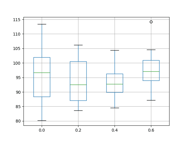
  Box and Whisker Plot of Recurrent Dropout Performance on the Shampoo Sales Dataset

  We can review how a recurrent dropout of 40% affects the dynamics of the model while being fit to the training data.

  The code below summarizes the updates to the fit_lstm() and run() functions compared to the baseline version of the diagnostic script.

  # fit an LSTM network to training data def fit_lstm(train, test, raw, scaler, batch_size, nb_epoch, neurons, dropout): X, y = train[:, 0:-1], train[:, -1] X = X.reshape(X.shape[0], 1, X.shape[1]) # prepare model model = Sequential() model.add(LSTM(neurons, batch_input_shape=(batch_size, X.shape[1], X.shape[2]), stateful=True, recurrent_dropout=dropout)) model.add(Dense(1)) model.compile(loss='mean_squared_error', optimizer='adam') # fit model train_rmse, test_rmse = list(), list() for i in range(nb_epoch): model.fit(X, y, epochs=1, batch_size=batch_size, verbose=0, shuffle=False) model.reset_states() # evaluate model on train data raw_train = raw[-(len(train)+len(test)+1):-len(test)] train_rmse.append(evaluate(model, raw_train, train, scaler, 0, batch_size)) # evaluate model on test data raw_test = raw[-(len(test)+1):] test_rmse.append(evaluate(model, raw_test, test, scaler, 0, batch_size)) history = DataFrame() history['train'], history['test'] = train_rmse, test_rmse return history   # run diagnostic experiments def run(): # config n_lag = 1 n_repeats = 10 n_epochs = 1000 n_batch = 4 n_neurons = 3 dropout = 0.4 # load dataset series = read_csv('shampoo-sales.csv', header=0, parse_dates=[0], index_col=0, squeeze=True, date_parser=parser) # transform data to be stationary raw_values = series.values diff_values = difference(raw_values, 1) # transform data to be supervised learning supervised = timeseries_to_supervised(diff_values, n_lag) supervised_values = supervised.values[n_lag:,:] # split data into train and test-sets train, test = supervised_values[0:-12], supervised_values[-12:] # transform the scale of the data scaler, train_scaled, test_scaled = scale(train, test) # fit and evaluate model train_trimmed = train_scaled[2:, :] # run diagnostic tests for i in range(n_repeats): history = fit_lstm(train_trimmed, test_scaled, raw_values, scaler, n_batch, n_epochs, n_neurons, dropout) pyplot.plot(history['train'], color='blue') pyplot.plot(history['test'], color='orange') print('%d) TrainRMSE=%f, TestRMSE=%f' % (i+1, history['train'].iloc[-1], history['test'].iloc[-1])) pyplot.savefig('diagnostic_dropout_recurrent.png')

  Running the updated diagnostic creates a plot of the train and test RMSE performance of the model with input dropout after each training epoch.

  The plot shows the addition of bumps on the test RMSE traces, with little effect on the training RMSE traces. The plot also suggests a plateau, if not an increasing trend in test RMSE after about 500 epochs.

  At least on this LSTM configuration and on this problem, perhaps recurrent dropout may not add much value.

  

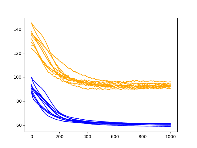
  Diagnostic Line Plot of Recurrent Dropout Performance on the Shampoo Sales Dataset

  Extensions

  This section lists some ideas for further experiments you might like to consider exploring after completing this tutorial.

  • Input Layer Dropout. It may be worth exploring the use of dropout on the input layer and how this impacts the performance and overfitting of the LSTM.
  • Combine Input and Recurrent. It may be worth exploring the combination of both input and recurrent dropout to see if any additional benefit can be provided.
  • Other Regularization Methods. It may be worth exploring other regularization methods with LSTM networks, such as various input, recurrent, and bias weight regularization functions.

  Further Reading

  For more on dropout with MLP models in Keras, see the post:

  • Dropout Regularization in Deep Learning Models With Keras

  Below are some papers on dropout with LSTM networks that you might find useful for further reading.

  • Recurrent Neural Network Regularization
  • A Theoretically Grounded Application of Dropout in Recurrent Neural Networks
  • Dropout improves Recurrent Neural Networks for Handwriting Recognition

  Summary

  In this tutorial, you discovered how to use dropout with LSTMs for time series forecasting.

  Specifically, you learned:

  • How to design a robust test harness for evaluating LSTM networks for time series forecasting.
  • How to configure input weight dropout on LSTMs for time series forecasting.
  • How to configure recurrent weight dropout on LSTMs for time series forecasting.

  Do you have any questions about using dropout with LSTM networks?
  Ask your questions in the comments below and I will do my best to answer.