How to Tune LSTM Hyperparameters with Keras for Time Series Forecasting

 Configuring neural networks is difficult because there is no good theory on how to do it.

You must be systematic and explore different configurations both from a dynamical and an objective results point of a view to try to understand what is going on for a given predictive modeling problem.

In this tutorial, you will discover how you can explore how to configure an LSTM network on a time series forecasting problem.

After completing this tutorial, you will know:

• How to tune and interpret the results of the number of training epochs.
• How to tune and interpret the results of the size of training batches.
• How to tune and interpret the results of the number of neurons.

  Tutorial Overview

  This tutorial is broken down into 6 parts; they are:

  1. Shampoo Sales Dataset
  2. Experimental Test Harness
  3. Tuning the Number of Epochs
  4. Tuning the Batch Size
  5. Tuning the Number of Neurons
  6. Summary of Results

  Environment

  This tutorial assumes you have a Python SciPy environment installed. You can use either Python 2 or 3 with this example.

  This tutorial assumes you have Keras v2.0 or higher installed with either the TensorFlow or Theano backend.

  The tutorial also assumes you have scikit-learn, Pandas, NumPy and Matplotlib installed.

  If you need help setting up your Python environment, see this post:

  • How to Setup a Python Environment for Machine Learning and Deep Learning with Anaconda

  Shampoo Sales Dataset

  This dataset describes the monthly number of sales of shampoo over a 3-year period.

  The units are a sales count and there are 36 observations. The original dataset is credited to Makridakis, Wheelwright, and Hyndman (1998).

  • Download the dataset.

  The example below loads and creates a plot of the loaded dataset.

  # load and plot dataset from pandas import read_csv from pandas import datetime from matplotlib import pyplot # load dataset def parser(x): return datetime.strptime('190'+x, '%Y-%m') series = read_csv('shampoo-sales.csv', header=0, parse_dates=[0], index_col=0, squeeze=True, date_parser=parser) # summarize first few rows print(series.head()) # line plot series.plot() pyplot.show()

  Running the example loads the dataset as a Pandas Series and prints the first 5 rows.

  Month 1901-01-01 266.0 1901-02-01 145.9 1901-03-01 183.1 1901-04-01 119.3 1901-05-01 180.3 Name: Sales, dtype: float64

  A line plot of the series is then created showing a clear increasing trend.

  

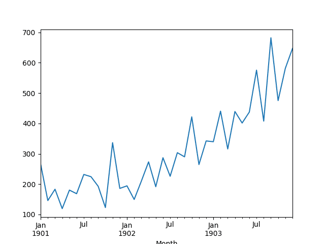
  Line Plot of Shampoo Sales Dataset

  Next, we will take a look at the LSTM configuration and test harness used in the experiment.

  Need help with Deep Learning for Time Series?

  Take my free 7-day email crash course now (with sample code).

  Click to sign-up and also get a free PDF Ebook version of the course.

  Experimental Test Harness

  This section describes the test harness used in this tutorial.

  Data Split

  We will split the Shampoo Sales dataset into two parts: a training and a test set.

  The first two years of data will be taken for the training dataset and the remaining one year of data will be used for the test set.

  Models will be developed using the training dataset and will make predictions on the test dataset.

  The persistence forecast (naive forecast) on the test dataset achieves an error of 136.761 monthly shampoo sales. This provides a lower acceptable bound of performance on the test set.

  Model Evaluation

  A rolling-forecast scenario will be used, also called walk-forward model validation.

  Each time step of the test dataset will be walked one at a time. A model will be used to make a forecast for the time step, then the actual expected value from the test set will be taken and made available to the model for the forecast on the next time step.

  This mimics a real-world scenario where new Shampoo Sales observations would be available each month and used in the forecasting of the following month.

  This will be simulated by the structure of the train and test datasets. We will make all of the forecasts in a one-shot method.

  All forecasts on the test dataset will be collected and an error score calculated to summarize the skill of the model. The root mean squared error (RMSE) will be used as it punishes large errors and results in a score that is in the same units as the forecast data, namely monthly shampoo sales.

  Data Preparation

  Before we can fit an LSTM model to the dataset, we must transform the data.

  The following three data transforms are performed on the dataset prior to fitting a model and making a forecast.

  1. Transform the time series data so that it is stationary. Specifically, a lag=1 differencing to remove the increasing trend in the data.
  2. Transform the time series into a supervised learning problem. Specifically, the organization of data into input and output patterns where the observation at the previous time step is used as an input to forecast the observation at the current time time step
  3. Transform the observations to have a specific scale. Specifically, to rescale the data to values between -1 and 1 to meet the default hyperbolic tangent activation function of the LSTM model.

  These transforms are inverted on forecasts to return them into their original scale before calculating and error score.

  Experimental Runs

  Each experimental scenario will be run 10 times.

  The reason for this is that the random initial conditions for an LSTM network can result in very different results each time a given configuration is trained.

  A diagnostic approach will be used to investigate model configurations. This is where line plots of model skill over time (training iterations called epochs) will be created and studied for insight into how a given configuration performs and how it may be adjusted to elicit better performance.

  The model will be evaluated on both the train and the test datasets at the end of each epoch and the RMSE scores saved.

  The train and test RMSE scores at the end of each scenario are printed to give an indication of progress.

  The series of train and test RMSE scores are plotted at the end of a run as a line plot. Train scores are colored blue and test scores are colored orange.

  Let’s dive into the results.

  Tuning the Number of Epochs

  The first LSTM parameter we will look at tuning is the number of training epochs.

  The model will use a batch size of 4, and a single neuron. We will explore the effect of training this configuration for different numbers of training epochs.

  Diagnostic of 500 Epochs

  The complete code listing for this diagnostic is listed below.

  The code is reasonably well commented and should be easy to follow. This code will be the basis for all future experiments in this tutorial and only the changes made in each subsequent experiment will be listed.

  from pandas import DataFrame from pandas import Series from pandas import concat from pandas import read_csv from pandas import datetime from sklearn.metrics import mean_squared_error from sklearn.preprocessing import MinMaxScaler from keras.models import Sequential from keras.layers import Dense from keras.layers import LSTM from math import sqrt import matplotlib # be able to save images on server matplotlib.use('Agg') from matplotlib import pyplot import numpy   # date-time parsing function for loading the dataset def parser(x): return datetime.strptime('190'+x, '%Y-%m')   # frame a sequence as a supervised learning problem def timeseries_to_supervised(data, lag=1): df = DataFrame(data) columns = [df.shift(i) for i in range(1, lag+1)] columns.append(df) df = concat(columns, axis=1) df = df.drop(0) return df   # create a differenced series def difference(dataset, interval=1): diff = list() for i in range(interval, len(dataset)): value = dataset[i] - dataset[i - interval] diff.append(value) return Series(diff)   # scale train and test data to [-1, 1] def scale(train, test): # fit scaler scaler = MinMaxScaler(feature_range=(-1, 1)) scaler = scaler.fit(train) # transform train train = train.reshape(train.shape[0], train.shape[1]) train_scaled = scaler.transform(train) # transform test test = test.reshape(test.shape[0], test.shape[1]) test_scaled = scaler.transform(test) return scaler, train_scaled, test_scaled   # inverse scaling for a forecasted value def invert_scale(scaler, X, yhat): new_row = [x for x in X] + [yhat] array = numpy.array(new_row) array = array.reshape(1, len(array)) inverted = scaler.inverse_transform(array) return inverted[0, -1]   # evaluate the model on a dataset, returns RMSE in transformed units def evaluate(model, raw_data, scaled_dataset, scaler, offset, batch_size): # separate X, y = scaled_dataset[:,0:-1], scaled_dataset[:,-1] # reshape reshaped = X.reshape(len(X), 1, 1) # forecast dataset output = model.predict(reshaped, batch_size=batch_size) # invert data transforms on forecast predictions = list() for i in range(len(output)): yhat = output[i,0] # invert scaling yhat = invert_scale(scaler, X[i], yhat) # invert differencing yhat = yhat + raw_data[i] # store forecast predictions.append(yhat) # report performance rmse = sqrt(mean_squared_error(raw_data[1:], predictions)) return rmse   # fit an LSTM network to training data def fit_lstm(train, test, raw, scaler, batch_size, nb_epoch, neurons): X, y = train[:, 0:-1], train[:, -1] X = X.reshape(X.shape[0], 1, X.shape[1]) # prepare model model = Sequential() model.add(LSTM(neurons, batch_input_shape=(batch_size, X.shape[1], X.shape[2]), stateful=True)) model.add(Dense(1)) model.compile(loss='mean_squared_error', optimizer='adam') # fit model train_rmse, test_rmse = list(), list() for i in range(nb_epoch): model.fit(X, y, epochs=1, batch_size=batch_size, verbose=0, shuffle=False) model.reset_states() # evaluate model on train data raw_train = raw[-(len(train)+len(test)+1):-len(test)] train_rmse.append(evaluate(model, raw_train, train, scaler, 0, batch_size)) model.reset_states() # evaluate model on test data raw_test = raw[-(len(test)+1):] test_rmse.append(evaluate(model, raw_test, test, scaler, 0, batch_size)) model.reset_states() history = DataFrame() history['train'], history['test'] = train_rmse, test_rmse return history   # run diagnostic experiments def run(): # load dataset series = read_csv('shampoo-sales.csv', header=0, parse_dates=[0], index_col=0, squeeze=True, date_parser=parser) # transform data to be stationary raw_values = series.values diff_values = difference(raw_values, 1) # transform data to be supervised learning supervised = timeseries_to_supervised(diff_values, 1) supervised_values = supervised.values # split data into train and test-sets train, test = supervised_values[0:-12], supervised_values[-12:] # transform the scale of the data scaler, train_scaled, test_scaled = scale(train, test) # fit and evaluate model train_trimmed = train_scaled[2:, :] # config repeats = 10 n_batch = 4 n_epochs = 500 n_neurons = 1 # run diagnostic tests for i in range(repeats): history = fit_lstm(train_trimmed, test_scaled, raw_values, scaler, n_batch, n_epochs, n_neurons) pyplot.plot(history['train'], color='blue') pyplot.plot(history['test'], color='orange') print('%d) TrainRMSE=%f, TestRMSE=%f' % (i, history['train'].iloc[-1], history['test'].iloc[-1])) pyplot.savefig('epochs_diagnostic.png')   # entry point run()

  Note: Your results may vary given the stochastic nature of the algorithm or evaluation procedure, or differences in numerical precision. Consider running the example a few times and compare the average outcome.

  Running the experiment prints the RMSE for the train and the test sets at the end of each of the 10 experimental runs.

  0) TrainRMSE=63.495594, TestRMSE=113.472643 1) TrainRMSE=60.446307, TestRMSE=100.147470 2) TrainRMSE=59.879681, TestRMSE=95.112331 3) TrainRMSE=66.115269, TestRMSE=106.444401 4) TrainRMSE=61.878702, TestRMSE=86.572920 5) TrainRMSE=73.519382, TestRMSE=103.551694 6) TrainRMSE=64.407033, TestRMSE=98.849227 7) TrainRMSE=72.684834, TestRMSE=98.499976 8) TrainRMSE=77.593773, TestRMSE=124.404747 9) TrainRMSE=71.749335, TestRMSE=126.396615

  A line plot of the series of RMSE scores on the train and test sets after each training epoch is also created.

  

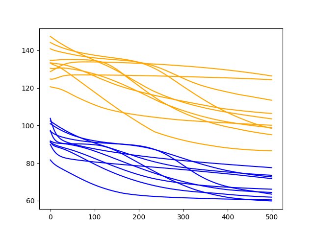
  Diagnostic Results with 500 Epochs

  The results clearly show a downward trend in RMSE over the training epochs for almost all of the experimental runs.

  This is a good sign, as it shows the model is learning the problem and has some predictive skill. In fact, all of the final test scores are below the error of a simple persistence model (naive forecast) that achieves an RMSE of 136.761 on this problem.

  The results suggest that more training epochs will result in a more skillful model.

  Let’s try doubling the number of epochs from 500 to 1000.

  Diagnostic of 1000 Epochs

  In this section, we use the same experimental setup and fit the model over 1000 training epochs.

  Specifically, the n_epochs parameter is set to 1000 in the run() function.

  n_epochs = 1000

  Note: Your results may vary given the stochastic nature of the algorithm or evaluation procedure, or differences in numerical precision. Consider running the example a few times and compare the average outcome.

  Running the example prints the RMSE for the train and test sets from the final epoch.

  0) TrainRMSE=69.242394, TestRMSE=90.832025 1) TrainRMSE=65.445810, TestRMSE=113.013681 2) TrainRMSE=57.949335, TestRMSE=103.727228 3) TrainRMSE=61.808586, TestRMSE=89.071392 4) TrainRMSE=68.127167, TestRMSE=88.122807 5) TrainRMSE=61.030678, TestRMSE=93.526607 6) TrainRMSE=61.144466, TestRMSE=97.963895 7) TrainRMSE=59.922150, TestRMSE=94.291120 8) TrainRMSE=60.170052, TestRMSE=90.076229 9) TrainRMSE=62.232470, TestRMSE=98.174839

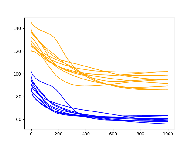
  A line plot of the test and train RMSE scores each epoch is also created.

  

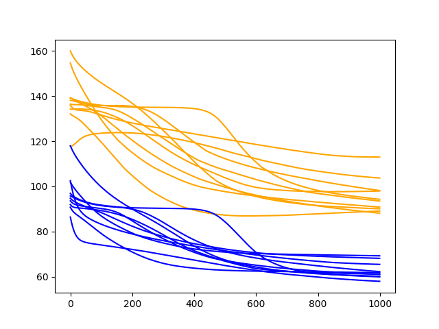
  Diagnostic Results with 1000 Epochs

  We can see that the downward trend of model error does continue and appears to slow.

  The lines for the train and test cases become more horizontal, but still generally show a downward trend, although at a lower rate of change. Some examples of test error show a possible inflection point around 600 epochs and may show a rising trend.

  It is worth extending the epochs further. We are interested in the average performance continuing to improve on the test set and this may continue.

  Let’s try doubling the number of epochs from 1000 to 2000.

  Diagnostic of 2000 Epochs

  In this section, we use the same experimental setup and fit the model over 2000 training epochs.

  Specifically, the n_epochs parameter is set to 2000 in the run() function.

  n_epochs = 2000

  Note: Your results may vary given the stochastic nature of the algorithm or evaluation procedure, or differences in numerical precision. Consider running the example a few times and compare the average outcome.

  Running the example prints the RMSE for the train and test sets from the final epoch.

  0) TrainRMSE=67.292970, TestRMSE=83.096856 1) TrainRMSE=55.098951, TestRMSE=104.211509 2) TrainRMSE=69.237206, TestRMSE=117.392007 3) TrainRMSE=61.319941, TestRMSE=115.868142 4) TrainRMSE=60.147575, TestRMSE=87.793270 5) TrainRMSE=59.424241, TestRMSE=99.000790 6) TrainRMSE=66.990082, TestRMSE=80.490660 7) TrainRMSE=56.467012, TestRMSE=97.799062 8) TrainRMSE=60.386380, TestRMSE=103.810569 9) TrainRMSE=58.250862, TestRMSE=86.212094

  A line plot of the test and train RMSE scores each epoch is also created.

  

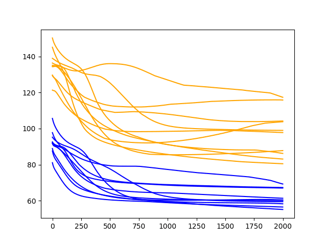
  Diagnostic Results with 2000 Epochs

  As one might have guessed, the downward trend in error continues over the additional 1000 epochs on both the train and test datasets.

  Of note, about half of the cases continue to decrease in error all the way to the end of the run, whereas the rest show signs of an increasing trend.

  The increasing trend is a sign of overfitting. This is when the model overfits the training dataset at the cost of worse performance on the test dataset. It is exemplified by continued improvements on the training dataset and improvements followed by an inflection point and worsting skill in the test dataset. A little less than half of the runs show the beginnings of this type of pattern on the test dataset.

  Nevertheless, the final epoch results on the test dataset are very good. If there is a chance we can see further gains by even longer training, we must explore it.

  Let’s try doubling the number of epochs from 2000 to 4000.

  Diagnostic of 4000 Epochs

  In this section, we use the same experimental setup and fit the model over 4000 training epochs.

  Specifically, the n_epochs parameter is set to 4000 in the run() function.

  n_epochs = 4000

  Note: Your results may vary given the stochastic nature of the algorithm or evaluation procedure, or differences in numerical precision. Consider running the example a few times and compare the average outcome.

  Running the example prints the RMSE for the train and test sets from the final epoch.

  0) TrainRMSE=58.889277, TestRMSE=99.121765 1) TrainRMSE=56.839065, TestRMSE=95.144846 2) TrainRMSE=58.522271, TestRMSE=87.671309 3) TrainRMSE=53.873962, TestRMSE=113.920076 4) TrainRMSE=66.386299, TestRMSE=77.523432 5) TrainRMSE=58.996230, TestRMSE=136.367014 6) TrainRMSE=55.725800, TestRMSE=113.206607 7) TrainRMSE=57.334604, TestRMSE=90.814642 8) TrainRMSE=54.593069, TestRMSE=105.724825 9) TrainRMSE=56.678498, TestRMSE=83.082262

  A line plot of the test and train RMSE scores each epoch is also created.

  

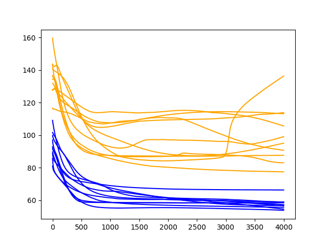
  Diagnostic Results with 4000 Epochs

  A similar pattern continues.

  There is a general trend of improving performance, even over the 4000 epochs. There is one case of severe overfitting where test error rises sharply.

  Again, most runs end with a “good” (better than persistence) final test error.

  Summary of Results

  The diagnostic runs above are helpful to explore the dynamical behavior of the model, but fall short of an objective and comparable mean performance.

  We can address this by repeating the same experiments and calculating and comparing summary statistics for each configuration. In this case, 30 runs were completed of the epoch values 500, 1000, 2000, 4000, and 6000.

  The idea is to compare the configurations using summary statistics over a larger number of runs and see exactly which of the configurations might perform better on average.

  The complete code example is listed below.

  from pandas import DataFrame from pandas import Series from pandas import concat from pandas import read_csv from pandas import datetime from sklearn.metrics import mean_squared_error from sklearn.preprocessing import MinMaxScaler from keras.models import Sequential from keras.layers import Dense from keras.layers import LSTM from math import sqrt import matplotlib # be able to save images on server matplotlib.use('Agg') from matplotlib import pyplot import numpy   # date-time parsing function for loading the dataset def parser(x): return datetime.strptime('190'+x, '%Y-%m')   # frame a sequence as a supervised learning problem def timeseries_to_supervised(data, lag=1): df = DataFrame(data) columns = [df.shift(i) for i in range(1, lag+1)] columns.append(df) df = concat(columns, axis=1) df = df.drop(0) return df   # create a differenced series def difference(dataset, interval=1): diff = list() for i in range(interval, len(dataset)): value = dataset[i] - dataset[i - interval] diff.append(value) return Series(diff)   # invert differenced value def inverse_difference(history, yhat, interval=1): return yhat + history[-interval]   # scale train and test data to [-1, 1] def scale(train, test): # fit scaler scaler = MinMaxScaler(feature_range=(-1, 1)) scaler = scaler.fit(train) # transform train train = train.reshape(train.shape[0], train.shape[1]) train_scaled = scaler.transform(train) # transform test test = test.reshape(test.shape[0], test.shape[1]) test_scaled = scaler.transform(test) return scaler, train_scaled, test_scaled   # inverse scaling for a forecasted value def invert_scale(scaler, X, yhat): new_row = [x for x in X] + [yhat] array = numpy.array(new_row) array = array.reshape(1, len(array)) inverted = scaler.inverse_transform(array) return inverted[0, -1]   # fit an LSTM network to training data def fit_lstm(train, batch_size, nb_epoch, neurons): X, y = train[:, 0:-1], train[:, -1] X = X.reshape(X.shape[0], 1, X.shape[1]) model = Sequential() model.add(LSTM(neurons, batch_input_shape=(batch_size, X.shape[1], X.shape[2]), stateful=True)) model.add(Dense(1)) model.compile(loss='mean_squared_error', optimizer='adam') for i in range(nb_epoch): model.fit(X, y, epochs=1, batch_size=batch_size, verbose=0, shuffle=False) model.reset_states() return model   # run a repeated experiment def experiment(repeats, series, epochs): # transform data to be stationary raw_values = series.values diff_values = difference(raw_values, 1) # transform data to be supervised learning supervised = timeseries_to_supervised(diff_values, 1) supervised_values = supervised.values # split data into train and test-sets train, test = supervised_values[0:-12], supervised_values[-12:] # transform the scale of the data scaler, train_scaled, test_scaled = scale(train, test) # run experiment error_scores = list() for r in range(repeats): # fit the model batch_size = 4 train_trimmed = train_scaled[2:, :] lstm_model = fit_lstm(train_trimmed, batch_size, epochs, 1) # forecast the entire training dataset to build up state for forecasting train_reshaped = train_trimmed[:, 0].reshape(len(train_trimmed), 1, 1) lstm_model.predict(train_reshaped, batch_size=batch_size) # forecast test dataset test_reshaped = test_scaled[:,0:-1] test_reshaped = test_reshaped.reshape(len(test_reshaped), 1, 1) output = lstm_model.predict(test_reshaped, batch_size=batch_size) predictions = list() for i in range(len(output)): yhat = output[i,0] X = test_scaled[i, 0:-1] # invert scaling yhat = invert_scale(scaler, X, yhat) # invert differencing yhat = inverse_difference(raw_values, yhat, len(test_scaled)+1-i) # store forecast predictions.append(yhat) # report performance rmse = sqrt(mean_squared_error(raw_values[-12:], predictions)) print('%d) Test RMSE: %.3f' % (r+1, rmse)) error_scores.append(rmse) return error_scores     # load dataset series = read_csv('shampoo-sales.csv', header=0, parse_dates=[0], index_col=0, squeeze=True, date_parser=parser) # experiment repeats = 30 results = DataFrame() # vary training epochs epochs = [500, 1000, 2000, 4000, 6000] for e in epochs: results[str(e)] = experiment(repeats, series, e) # summarize results print(results.describe()) # save boxplot results.boxplot() pyplot.savefig('boxplot_epochs.png')

  Running the code first prints summary statistics for each of the 5 configurations. Notably, this includes the mean and standard deviations of the RMSE scores from each population of results.

  Note: Your results may vary given the stochastic nature of the algorithm or evaluation procedure, or differences in numerical precision. Consider running the example a few times and compare the average outcome.

  The mean gives an idea of the average expected performance of a configuration, whereas the standard deviation gives an idea of the variance. The min and max RMSE scores also give an idea of the range of possible best and worst case examples that might be expected.

  Looking at just the mean RMSE scores, the results suggest that an epoch configured to 1000 may be better. The results also suggest further investigations may be warranted of epoch values between 1000 and 2000.

  500        1000        2000        4000        6000 count   30.000000   30.000000   30.000000   30.000000   30.000000 mean   109.439203  104.566259  107.882390  116.339792  127.618305 std     14.874031   19.097098   22.083335   21.590424   24.866763 min     87.747708   81.621783   75.327883   77.399968   90.512409 25%     96.484568   87.686776   86.753694  102.127451  105.861881 50%    110.891939   98.942264  116.264027  121.898248  125.273050 75%    121.067498  119.248849  125.518589  130.107772  150.832313 max    138.879278  139.928055  146.840997  157.026562  166.111151

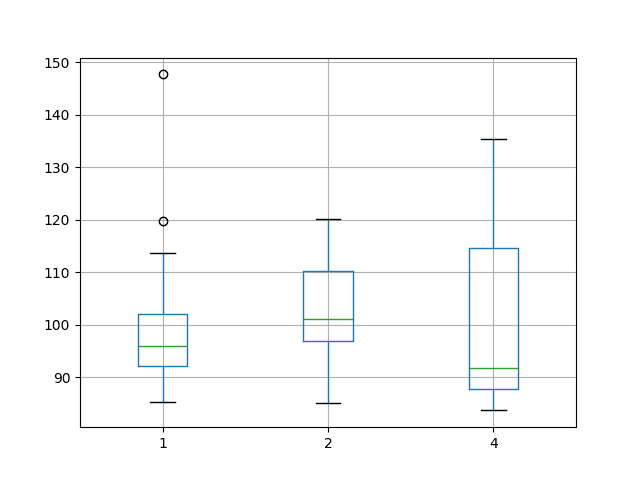
  The distributions are also shown on a box and whisker plot. This is helpful to see how the distributions directly compare.

  The green line shows the median and the box shows the 25th and 75th percentiles, or the middle 50% of the data. This comparison also shows that the choice of setting epochs to 1000 is better than the tested alternatives. It also shows that the best possible performance may be achieved with epochs of 2000 or 4000, at the cost of worse performance on average.

  

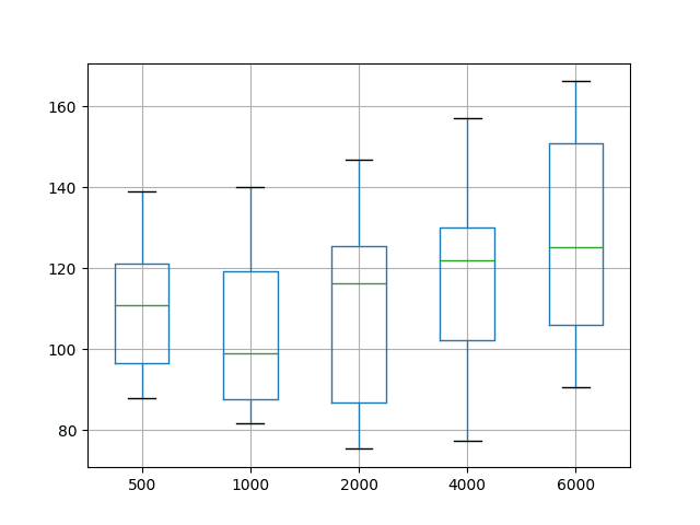
  Box and Whisker Plot Summarizing Epoch Results

  Next, we will look at the effect of batch size.

  Tuning the Batch Size

  Batch size controls how often to update the weights of the network.

  Importantly in Keras, the batch size must be a factor of the size of the test and the training dataset.

  In the previous section exploring the number of training epochs, the batch size was fixed at 4, which cleanly divides into the test dataset (with the size 12) and in a truncated version of the test dataset (with the size of 20).

  In this section, we will explore the effect of varying the batch size. We will hold the number of training epochs constant at 1000.

  Diagnostic of 1000 Epochs and Batch Size of 4

  As a reminder, the previous section evaluated a batch size of 4 in the second experiment with a number of epochs of 1000.

  The results showed a downward trend in error that continued for most runs all the way to the final training epoch.

  

  Diagnostic Results with 1000 Epochs

  Diagnostic of 1000 Epochs and Batch Size of 2

  In this section, we look at halving the batch size from 4 to 2.

  This change is made to the n_batch parameter in the run() function; for example:

  n_batch = 2

  Running the example shows the same general trend in performance as a batch size of 4, perhaps with a higher RMSE on the final epoch.

  Note: Your results may vary given the stochastic nature of the algorithm or evaluation procedure, or differences in numerical precision. Consider running the example a few times and compare the average outcome.

  The runs may show the behavior of stabilizing the RMES sooner rather than seeming to continue the downward trend.

  The RSME scores from the final exposure of each run are listed below.

  0) TrainRMSE=63.510219, TestRMSE=115.855819 1) TrainRMSE=58.336003, TestRMSE=97.954374 2) TrainRMSE=69.163685, TestRMSE=96.721446 3) TrainRMSE=65.201764, TestRMSE=110.104828 4) TrainRMSE=62.146057, TestRMSE=112.153553 5) TrainRMSE=58.253952, TestRMSE=98.442715 6) TrainRMSE=67.306530, TestRMSE=108.132021 7) TrainRMSE=63.545292, TestRMSE=102.821356 8) TrainRMSE=61.693847, TestRMSE=99.859398 9) TrainRMSE=58.348250, TestRMSE=99.682159

  A line plot of the test and train RMSE scores each epoch is also created.

  

  Diagnostic Results with 1000 Epochs and Batch Size of 2

  Let’s try having the batch size again.

  Diagnostic of 1000 Epochs and Batch Size of 1

  A batch size of 1 is technically performing online learning.

  That is where the network is updated after each training pattern. This can be contrasted with batch learning, where the weights are only updated at the end of each epoch.

  We can change the n_batch parameter in the run() function; for example:

  n_batch = 1

  Note: Your results may vary given the stochastic nature of the algorithm or evaluation procedure, or differences in numerical precision. Consider running the example a few times and compare the average outcome.

  Again, running the example prints the RMSE scores from the final epoch of each run.

  0) TrainRMSE=60.349798, TestRMSE=100.182293 1) TrainRMSE=62.624106, TestRMSE=95.716070 2) TrainRMSE=64.091859, TestRMSE=98.598958 3) TrainRMSE=59.929993, TestRMSE=96.139427 4) TrainRMSE=59.890593, TestRMSE=94.173619 5) TrainRMSE=55.944968, TestRMSE=106.644275 6) TrainRMSE=60.570245, TestRMSE=99.981562 7) TrainRMSE=56.704995, TestRMSE=111.404182 8) TrainRMSE=59.909065, TestRMSE=90.238473 9) TrainRMSE=60.863807, TestRMSE=105.331214

  A line plot of the test and train RMSE scores each epoch is also created.

  The plot suggests more variability in the test RMSE over time and perhaps a train RMSE that stabilizes sooner than with larger batch sizes. The increased variability in the test RMSE is to be expected given the large changes made to the network give so little feedback each update.

  The graph also suggests that perhaps the decreasing trend in RMSE may continue if the configuration was afforded more training epochs.

  

  Diagnostic Results with 1000 Epochs and Batch Size of 1

  Summary of Results

  As with training epochs, we can objectively compare the performance of the network given different batch sizes.

  Each configuration was run 30 times and summary statistics calculated on the final results.

  ...   # run a repeated experiment def experiment(repeats, series, batch_size): # transform data to be stationary raw_values = series.values diff_values = difference(raw_values, 1) # transform data to be supervised learning supervised = timeseries_to_supervised(diff_values, 1) supervised_values = supervised.values # split data into train and test-sets train, test = supervised_values[0:-12], supervised_values[-12:] # transform the scale of the data scaler, train_scaled, test_scaled = scale(train, test) # run experiment error_scores = list() for r in range(repeats): # fit the model train_trimmed = train_scaled[2:, :] lstm_model = fit_lstm(train_trimmed, batch_size, 1000, 1) # forecast the entire training dataset to build up state for forecasting train_reshaped = train_trimmed[:, 0].reshape(len(train_trimmed), 1, 1) lstm_model.predict(train_reshaped, batch_size=batch_size) # forecast test dataset test_reshaped = test_scaled[:,0:-1] test_reshaped = test_reshaped.reshape(len(test_reshaped), 1, 1) output = lstm_model.predict(test_reshaped, batch_size=batch_size) predictions = list() for i in range(len(output)): yhat = output[i,0] X = test_scaled[i, 0:-1] # invert scaling yhat = invert_scale(scaler, X, yhat) # invert differencing yhat = inverse_difference(raw_values, yhat, len(test_scaled)+1-i) # store forecast predictions.append(yhat) # report performance rmse = sqrt(mean_squared_error(raw_values[-12:], predictions)) print('%d) Test RMSE: %.3f' % (r+1, rmse)) error_scores.append(rmse) return error_scores     # load dataset series = read_csv('shampoo-sales.csv', header=0, parse_dates=[0], index_col=0, squeeze=True, date_parser=parser) # experiment repeats = 30 results = DataFrame() # vary training batches batches = [1, 2, 4] for b in batches: results[str(b)] = experiment(repeats, series, b) # summarize results print(results.describe()) # save boxplot results.boxplot() pyplot.savefig('boxplot_batches.png')

  Note: Your results may vary given the stochastic nature of the algorithm or evaluation procedure, or differences in numerical precision. Consider running the example a few times and compare the average outcome.

  From the mean performance alone, the results suggest lower RMSE with a batch size of 1. As was noted in the previous section, this may be improved further with more training epochs.

  1           2           4 count   30.000000   30.000000   30.000000 mean    98.697017  102.642594  100.320203 std     12.227885    9.144163   15.957767 min     85.172215   85.072441   83.636365 25%     92.023175   96.834628   87.671461 50%     95.981688  101.139527   91.628144 75%    102.009268  110.171802  114.660192 max    147.688818  120.038036  135.290829

  A box and whisker plot of the data was also created to help graphically compare the distributions. The plot shows the median performance as a green line where a batch size of 4 shows both the largest variability and also the lowest median RMSE.

  Tuning a neural network is a tradeoff of average performance and variability of that performance, with an ideal result having a low mean error with low variability, meaning that it is generally good and reproducible.

  

  Box and Whisker Plot Summarizing Batch Size Results

  Tuning the Number of Neurons

  In this section, we will investigate the effect of varying the number of neurons in the network.

  The number of neurons affects the learning capacity of the network. Generally, more neurons would be able to learn more structure from the problem at the cost of longer training time. More learning capacity also creates the problem of potentially overfitting the training data.

  We will use a batch size of 4 and 1000 training epochs.

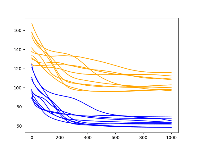
  Diagnostic of 1000 Epochs and 1 Neuron

  We will start with 1 neuron.

  As a reminder, this is the second configuration tested from the epochs experiments.

  

  Diagnostic Results with 1000 Epochs

  Diagnostic of 1000 Epochs and 2 Neurons

  We can increase the number of neurons from 1 to 2. This would be expected to improve the learning capacity of the network.

  We can do this by changing the n_neurons variable in the run() function.

  n_neurons = 2

  Running this configuration prints the RMSE scores from the final epoch of each run.

  Note: Your results may vary given the stochastic nature of the algorithm or evaluation procedure, or differences in numerical precision. Consider running the example a few times and compare the average outcome.

  The results suggest a good, but not great, general performance.

  0) TrainRMSE=59.466223, TestRMSE=95.554547 1) TrainRMSE=58.752515, TestRMSE=101.908449 2) TrainRMSE=58.061139, TestRMSE=86.589039 3) TrainRMSE=55.883708, TestRMSE=94.747927 4) TrainRMSE=58.700290, TestRMSE=86.393213 5) TrainRMSE=60.564511, TestRMSE=101.956549 6) TrainRMSE=63.160916, TestRMSE=98.925108 7) TrainRMSE=60.148595, TestRMSE=95.082825 8) TrainRMSE=63.029242, TestRMSE=89.285092 9) TrainRMSE=57.794717, TestRMSE=91.425071

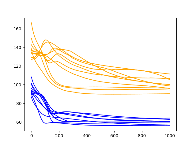
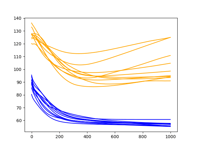
  A line plot of the test and train RMSE scores each epoch is also created.

  This is more telling. It shows a rapid decrease in test RMSE to about epoch 500-750 where an inflection point shows a rise in test RMSE almost across the board on all runs. Meanwhile, the training dataset shows a continued decrease to the final epoch.

  These are good signs of overfitting of the training dataset.

  

  Diagnostic Results with 1000 Epochs and 2 Neurons

  Let’s see if this trend continues with even more neurons.

  Diagnostic of 1000 Epochs and 3 Neurons

  This section looks at the same configuration with the number of neurons increased to 3.

  We can do this by setting the n_neurons variable in the run() function.

  n_neurons = 3

  Running this configuration prints the RMSE scores from the final epoch of each run.

  Note: Your results may vary given the stochastic nature of the algorithm or evaluation procedure, or differences in numerical precision. Consider running the example a few times and compare the average outcome.

  The results are similar to the previous section; we do not see much general difference between the final epoch test scores for 2 or 3 neurons. The final train scores do appear to be lower with 3 neurons, perhaps showing an acceleration of overfitting.

  The inflection point in the training dataset seems to be happening sooner than the 2 neurons experiment, perhaps at epoch 300-400.

  These increases in the number of neurons may benefit from additional changes to slowing down the rate of learning. Such as the use of regularization methods like dropout, decrease to the batch size, and decrease to the number of training epochs.

  0) TrainRMSE=55.686242, TestRMSE=90.955555 1) TrainRMSE=55.198617, TestRMSE=124.989622 2) TrainRMSE=55.767668, TestRMSE=104.751183 3) TrainRMSE=60.716046, TestRMSE=93.566307 4) TrainRMSE=57.703663, TestRMSE=110.813226 5) TrainRMSE=56.874231, TestRMSE=98.588524 6) TrainRMSE=57.206756, TestRMSE=94.386134 7) TrainRMSE=55.770377, TestRMSE=124.949862 8) TrainRMSE=56.876467, TestRMSE=95.059656 9) TrainRMSE=57.067810, TestRMSE=94.123620

  A line plot of the test and train RMSE scores each epoch is also created.

  

  Diagnostic Results with 1000 Epochs and 3 Neurons

  Summary of Results

  Again, we can objectively compare the impact of increasing the number of neurons while keeping all other network configurations fixed.

  In this section, we repeat each experiment 30 times and compare the average test RMSE performance with the number of neurons ranging from 1 to 5.

  ...   # run a repeated experiment def experiment(repeats, series, neurons): # transform data to be stationary raw_values = series.values diff_values = difference(raw_values, 1) # transform data to be supervised learning supervised = timeseries_to_supervised(diff_values, 1) supervised_values = supervised.values # split data into train and test-sets train, test = supervised_values[0:-12], supervised_values[-12:] # transform the scale of the data scaler, train_scaled, test_scaled = scale(train, test) # run experiment error_scores = list() for r in range(repeats): # fit the model batch_size = 4 train_trimmed = train_scaled[2:, :] lstm_model = fit_lstm(train_trimmed, batch_size, 1000, neurons) # forecast the entire training dataset to build up state for forecasting train_reshaped = train_trimmed[:, 0].reshape(len(train_trimmed), 1, 1) lstm_model.predict(train_reshaped, batch_size=batch_size) # forecast test dataset test_reshaped = test_scaled[:,0:-1] test_reshaped = test_reshaped.reshape(len(test_reshaped), 1, 1) output = lstm_model.predict(test_reshaped, batch_size=batch_size) predictions = list() for i in range(len(output)): yhat = output[i,0] X = test_scaled[i, 0:-1] # invert scaling yhat = invert_scale(scaler, X, yhat) # invert differencing yhat = inverse_difference(raw_values, yhat, len(test_scaled)+1-i) # store forecast predictions.append(yhat) # report performance rmse = sqrt(mean_squared_error(raw_values[-12:], predictions)) print('%d) Test RMSE: %.3f' % (r+1, rmse)) error_scores.append(rmse) return error_scores     # load dataset series = read_csv('shampoo-sales.csv', header=0, parse_dates=[0], index_col=0, squeeze=True, date_parser=parser) # experiment repeats = 30 results = DataFrame() # vary neurons neurons = [1, 2, 3, 4, 5] for n in neurons: results[str(n)] = experiment(repeats, series, n) # summarize results print(results.describe()) # save boxplot results.boxplot() pyplot.savefig('boxplot_neurons.png')

  Running the experiment prints the summary statistics for each configuration.

  Note: Your results may vary given the stochastic nature of the algorithm or evaluation procedure, or differences in numerical precision. Consider running the example a few times and compare the average outcome.

  From the mean performance alone, the results suggest a network configuration with 1 neuron as having the best performance over 1000 epochs with a batch size of 4. This configuration also shows the tightest variance.

  1           2           3           4           5 count   30.000000   30.000000   30.000000   30.000000   30.000000 mean    98.344696  103.268147  102.726894  112.453766  122.843032 std     13.538599   14.720989   12.905631   16.296657   25.586013 min     81.764721   87.731385   77.545899   85.632492   85.955093 25%     88.524334   94.040807   95.152752  102.477366  104.192588 50%     93.543948  100.330678  103.622600  110.906970  117.022724 75%    102.944050  105.087384  110.235754  118.653850  133.343669 max    132.934054  152.588092  130.551521  162.889845  184.678185

  The box and whisker plot shows a clear trend in the median test set performance where the increase in neurons results in a corresponding increase in the test RMSE.

  

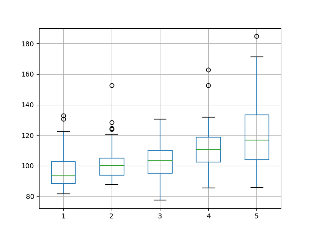
  Box and Whisker Plot Summarizing Neuron Results

  Summary of All Results

  We completed quite a few LSTM experiments on the Shampoo Sales dataset in this tutorial.

  Generally, it seems that a stateful LSTM configured with 1 neuron, a batch size of 4, and trained for 1000 epochs might be a good configuration.

  The results also suggest that perhaps this configuration with a batch size of 1 and fit for more epochs may be worthy of further exploration.

  Tuning neural networks is difficult empirical work, and LSTMs are proving to be no exception.

  This tutorial demonstrated the benefit of both diagnostic studies of configuration behavior over time, as well as objective studies of test RMSE.

  Nevertheless, there are always more studies that could be performed. Some ideas are listed in the next section.

  Extensions

  This section lists some ideas for extensions to the experiments performed in this tutorial.

  If you explore any of these, report your results in the comments; I’d love to see what you come up with.

  • Dropout. Slow down learning with regularization methods like dropout on the recurrent LSTM connections.
  • Layers. Explore additional hierarchical learning capacity by adding more layers and varied numbers of neurons in each layer.
  • Regularization. Explore how weight regularization, such as L1 and L2, can be used to slow down learning and overfitting of the network on some configurations.
  • Optimization Algorithm. Explore the use of alternate optimization algorithms, such as classical gradient descent, to see if specific configurations to speed up or slow down learning can lead to benefits.
  • Loss Function. Explore the use of alternative loss functions to see if these can be used to lift performance.
  • Features and Timesteps. Explore the use of lag observations as input features and input time steps of the feature to see if their presence as input can improve learning and/or predictive capability of the model.
  • Larger Batch Size. Explore larger batch sizes than 4, perhaps requiring further manipulation of the size of the training and test datasets.

  Summary

  In this tutorial, you discovered how you can systematically investigate the configuration for an LSTM network for time series forecasting.

  Specifically, you learned:

  • How to design a systematic test harness for evaluating model configurations.
  • How to use model diagnostics over time, as well as objective prediction error to interpret model behavior.
  • How to explore and interpret the effects of the number of training epochs, batch size, and number of neurons.

  Do you have any questions about tuning LSTMs, or about this tutorial?
  Ask your questions in the comments below and I will do my best to answer.