How to Load and Explore Time Series Data in Python

 The Pandas library in Python provides excellent, built-in support for time series data.

Once loaded, Pandas also provides tools to explore and better understand your dataset.

In this post, you will discover how to load and explore your time series dataset.

After completing this tutorial, you will know:

• How to load your time series dataset from a CSV file using Pandas.
• How to peek at the loaded data and calculate summary statistics.
• How to plot and review your time series data.

Kick-start your project with my new book Time Series Forecasting With Python, including step-by-step tutorials and the Python source code files for all examples.

Let’s get started.

• Updated Apr/2019: Updated the link to dataset.
• Update Aug/2019: Updated data loading to use new API.

Daily Female Births Dataset

In this post, we will use the Daily Female Births Dataset as an example.

This univariate time series dataset describes the number of daily female births in California in 1959.

The units are a count and there are 365 observations. The source of the dataset is credited to Newton (1988).

• Download the dataset.

Below is a sample of the first 5 rows of data, including the header row.

"Date","Daily total female births in California, 1959" "1959-01-01",35 "1959-01-02",32 "1959-01-03",30 "1959-01-04",31 "1959-01-05",44

Below is a plot of the entire dataset.

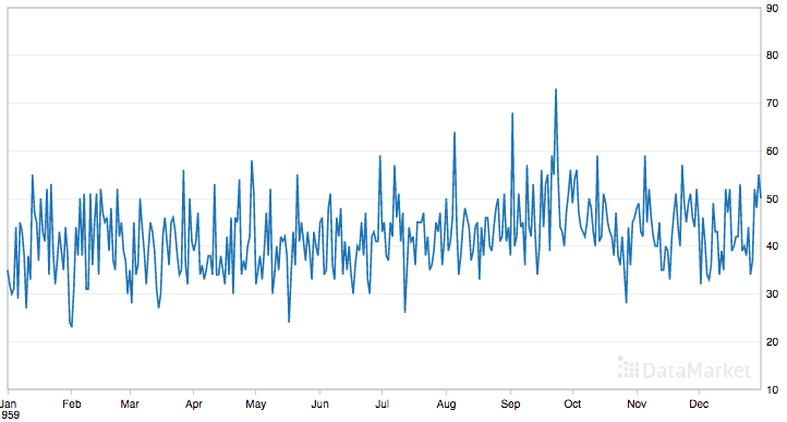
Daily Female Births Dataset

Download the dataset and place it in your current working directory with the file name “daily-total-female-births-in-cal.csv“.

• Download the dataset.

Load Time Series Data

Pandas represented time series datasets as a Series.

A Series is a one-dimensional array with a time label for each row.

The series has a name, which is the column name of the data column.

You can see that each row has an associated date. This is in fact not a column, but instead a time index for value. As an index, there can be multiple values for one time, and values may be spaced evenly or unevenly across times.

The main function for loading CSV data in Pandas is the read_csv() function. We can use this to load the time series as a Series object, instead of a DataFrame, as follows:

# Load birth data using read_csv from pandas import read_csv series = read_csv('daily-total-female-births-in-cal.csv', header=0, parse_dates=[0], index_col=0, squeeze=True) print(type(series)) print(series.head())

Note the arguments to the read_csv() function.

We provide it a number of hints to ensure the data is loaded as a Series.

• header=0: We must specify the header information at row 0.
• parse_dates=[0]: We give the function a hint that data in the first column contains dates that need to be parsed. This argument takes a list, so we provide it a list of one element, which is the index of the first column.
• index_col=0: We hint that the first column contains the index information for the time series.
• squeeze=True: We hint that we only have one data column and that we are interested in a Series and not a DataFrame.

One more argument you may need to use for your own data is date_parser to specify the function to parse date-time values. In this example, the date format has been inferred, and this works in most cases. In those few cases where it does not, specify your own date parsing function and use the date_parser argument.

Running the example above prints the same output, but also confirms that the time series was indeed loaded as a Series object.

<class 'pandas.core.series.Series'> Date 1959-01-01 35 1959-01-02 32 1959-01-03 30 1959-01-04 31 1959-01-05 44 Name: Daily total female births in California, 1959, dtype: int64

It is often easier to perform manipulations of your time series data in a DataFrame rather than a Series object.

In those situations, you can easily convert your loaded Series to a DataFrame as follows:

dataframe = DataFrame(series)

Further Reading

• More on the pandas.read_csv() function.

Stop learning Time Series Forecasting the slow way!

Take my free 7-day email course and discover how to get started (with sample code).

Click to sign-up and also get a free PDF Ebook version of the course.

Exploring Time Series Data

Pandas also provides tools to explore and summarize your time series data.

In this section, we’ll take a look at a few, common operations to explore and summarize your loaded time series data.

Peek at the Data

It is a good idea to take a peek at your loaded data to confirm that the types, dates, and data loaded as you intended.

You can use the head() function to peek at the first 5 records or specify the first n number of records to review.

For example, you can print the first 10 rows of data as follows.

from pandas import read_csv series = read_csv('daily-total-female-births-in-cal.csv', header=0, index_col=0) print(series.head(10))

Running the example prints the following:

Date 1959-01-01 35 1959-01-02 32 1959-01-03 30 1959-01-04 31 1959-01-05 44 1959-01-06 29 1959-01-07 45 1959-01-08 43 1959-01-09 38 1959-01-10 27

You can also use the tail() function to get the last n records of the dataset.

Number of Observations

Another quick check to perform on your data is the number of loaded observations.

This can help flush out issues with column headers not being handled as intended, and to get an idea on how to effectively divide up data later for use with supervised learning algorithms.

You can get the dimensionality of your Series using the size parameter.

from pandas import read_csv series = read_csv('daily-total-female-births-in-cal.csv', header=0, index_col=0) print(series.size)

Running this example we can see that as we would expect, there are 365 observations, one for each day of the year in 1959.

365

Querying By Time

You can slice, dice, and query your series using the time index.

For example, you can access all observations in January as follows:

from pandas import read_csv series = read_csv('daily-total-female-births-in-cal.csv', header=0, parse_dates=[0], index_col=0, squeeze=True) print(series['1959-01'])

Running this displays the 31 observations for the month of January in 1959.

Date 1959-01-01 35 1959-01-02 32 1959-01-03 30 1959-01-04 31 1959-01-05 44 1959-01-06 29 1959-01-07 45 1959-01-08 43 1959-01-09 38 1959-01-10 27 1959-01-11 38 1959-01-12 33 1959-01-13 55 1959-01-14 47 1959-01-15 45 1959-01-16 37 1959-01-17 50 1959-01-18 43 1959-01-19 41 1959-01-20 52 1959-01-21 34 1959-01-22 53 1959-01-23 39 1959-01-24 32 1959-01-25 37 1959-01-26 43 1959-01-27 39 1959-01-28 35 1959-01-29 44 1959-01-30 38 1959-01-31 24

This type of index-based querying can help to prepare summary statistics and plots while exploring the dataset.

Descriptive Statistics

Calculating descriptive statistics on your time series can help get an idea of the distribution and spread of values.

This may help with ideas of data scaling and even data cleaning that you can perform later as part of preparing your dataset for modeling.

The describe() function creates a 7 number summary of the loaded time series including mean, standard deviation, median, minimum, and maximum of the observations.

from pandas import read_csv series = read_csv('daily-total-female-births-in-cal.csv', header=0, index_col=0) print(series.describe())

Running this example prints a summary of the birth rate dataset.

count 365.000000 mean 41.980822 std 7.348257 min 23.000000 25% 37.000000 50% 42.000000 75% 46.000000 max 73.000000

Plotting Time Series

Plotting time series data, especially univariate time series, is an important part of exploring your data.

This functionality is provided on the loaded Series by calling the plot() function.

Below is an example of plotting the entire loaded time series dataset.

from pandas import read_csv from matplotlib import pyplot series = read_csv('daily-total-female-births-in-cal.csv', header=0, index_col=0) pyplot.plot(series) pyplot.show()

Running the example creates a time series plot with the number of daily births on the y-axis and time in days along the x-axis.

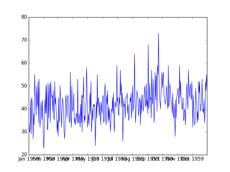
Daily Total Female Births Plot

Further Reading

If you’re interested in learning more about Pandas’ functionality working with time series data, see some of the links below.

• Pandas Time Series / Date functionality
• Pandas Time Series Basics
• Time series analysis with pandas

Summary

In this post, you discovered how to load and handle time series data using the Pandas Python library.

Specifically, you learned:

• How to load your time series data as a Pandas Series.
• How to peek at and calculate summary statistics of your time series data.
• How to plot your time series data.

Do you have any questions about handling time series data in Python, or about this post?
Ask your questions in the comments below and I will do my best to answer.