How To Implement Simple Linear Regression From Scratch With Python

 Linear regression is a prediction method that is more than 200 years old.

Simple linear regression is a great first machine learning algorithm to implement as it requires you to estimate properties from your training dataset, but is simple enough for beginners to understand.

In this tutorial, you will discover how to implement the simple linear regression algorithm from scratch in Python.

After completing this tutorial you will know:

• How to estimate statistical quantities from training data.
• How to estimate linear regression coefficients from data.
• How to make predictions using linear regression for new data.

  Description

  This section is divided into two parts, a description of the simple linear regression technique and a description of the dataset to which we will later apply it.

  Simple Linear Regression

  Linear regression assumes a linear or straight line relationship between the input variables (X) and the single output variable (y).

  More specifically, that output (y) can be calculated from a linear combination of the input variables (X). When there is a single input variable, the method is referred to as a simple linear regression.

  In simple linear regression we can use statistics on the training data to estimate the coefficients required by the model to make predictions on new data.

  The line for a simple linear regression model can be written as:

  y = b0 + b1 * x

  where b0 and b1 are the coefficients we must estimate from the training data.

  Once the coefficients are known, we can use this equation to estimate output values for y given new input examples of x.

  It requires that you calculate statistical properties from the data such as mean, variance and covariance.

  All the algebra has been taken care of and we are left with some arithmetic to implement to estimate the simple linear regression coefficients.

  Briefly, we can estimate the coefficients as follows:

  B1 = sum((x(i) - mean(x)) * (y(i) - mean(y))) / sum( (x(i) - mean(x))^2 ) B0 = mean(y) - B1 * mean(x)

  where the i refers to the value of the ith value of the input x or output y.

  Don’t worry if this is not clear right now, these are the functions will implement in the tutorial.

  Swedish Insurance Dataset

  We will use a real dataset to demonstrate simple linear regression.

  The dataset is called the “Auto Insurance in Sweden” dataset and involves predicting the total payment for all the claims in thousands of Swedish Kronor (y) given the total number of claims (x).

  This means that for a new number of claims (x) we will be able to predict the total payment of claims (y).

  Here is a small sample of the first 5 records of the dataset.

  108,392.5 19,46.2 13,15.7 124,422.2 40,119.4

  Using the Zero Rule algorithm (that predicts the mean value) a Root Mean Squared Error or RMSE of about 81 (thousands of Kronor) is expected.

  Below is a scatter plot of the entire dataset.

  

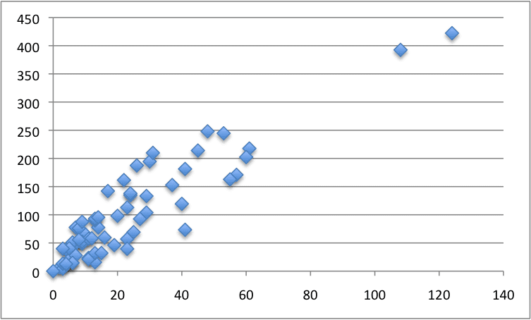
  Swedish Insurance Dataset

  You can download the raw dataset from here or here.

  Save it to a CSV file in your local working directory with the name “insurance.csv“.

  Note, you may need to convert the European “,” to the decimal “.”. You will also need change the file from white-space-separated variables to CSV format.

  Tutorial

  This tutorial is broken down into five parts:

  1. Calculate Mean and Variance.
  2. Calculate Covariance.
  3. Estimate Coefficients.
  4. Make Predictions.
  5. Predict Insurance.

  These steps will give you the foundation you need to implement and train simple linear regression models for your own prediction problems.

  1. Calculate Mean and Variance

  The first step is to estimate the mean and the variance of both the input and output variables from the training data.

  The mean of a list of numbers can be calculated as:

  mean(x) = sum(x) / count(x)

  Below is a function named mean() that implements this behavior for a list of numbers.

  # Calculate the mean value of a list of numbers def mean(values): return sum(values) / float(len(values))

  The variance is the sum squared difference for each value from the mean value.

  Variance for a list of numbers can be calculated as:

  variance = sum( (x - mean(x))^2 )

  Below is a function named variance() that calculates the sample variance of a list of numbers (Note that we are intentionally calculating the sum squared difference from the mean, instead of the average squared difference from the mean). It requires the mean of the list to be provided as an argument, just so we don’t have to calculate it more than once.

  # Calculate the variance of a list of numbers def variance(values, mean): return sum([(x-mean)**2 for x in values])

  We can put these two functions together and test them on a small contrived dataset.

  Below is a small dataset of x and y values.

  NOTE: delete the column headers from this data if you save it to a .CSV file for use with the final code example.

  x, y 1, 1 2, 3 4, 3 3, 2 5, 5

  We can plot this dataset on a scatter plot graph as follows:

  

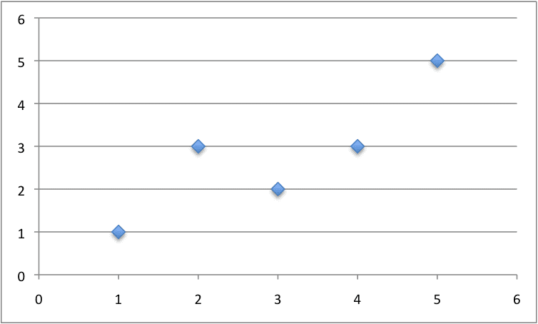
  Small Contrived Dataset For Simple Linear Regression

  We can calculate the mean and variance for both the x and y values in the example below.

  # Estimate Mean and Variance   # Calculate the mean value of a list of numbers def mean(values): return sum(values) / float(len(values))   # Calculate the variance of a list of numbers def variance(values, mean): return sum([(x-mean)**2 for x in values])   # calculate mean and variance dataset = [[1, 1], [2, 3], [4, 3], [3, 2], [5, 5]] x = [row[0] for row in dataset] y = [row[1] for row in dataset] mean_x, mean_y = mean(x), mean(y) var_x, var_y = variance(x, mean_x), variance(y, mean_y) print('x stats: mean=%.3f variance=%.3f' % (mean_x, var_x)) print('y stats: mean=%.3f variance=%.3f' % (mean_y, var_y))

  Running this example prints out the mean and variance for both columns.

  x stats: mean=3.000 variance=10.000 y stats: mean=2.800 variance=8.800

  This is our first step, next we need to put these values to use in calculating the covariance.

  2. Calculate Covariance

  The covariance of two groups of numbers describes how those numbers change together.

  Covariance is a generalization of correlation. Correlation describes the relationship between two groups of numbers, whereas covariance can describe the relationship between two or more groups of numbers.

  Additionally, covariance can be normalized to produce a correlation value.

  Nevertheless, we can calculate the covariance between two variables as follows:

  covariance = sum((x(i) - mean(x)) * (y(i) - mean(y)))

  Below is a function named covariance() that implements this statistic. It builds upon the previous step and takes the lists of x and y values as well as the mean of these values as arguments.

  # Calculate covariance between x and y def covariance(x, mean_x, y, mean_y): covar = 0.0 for i in range(len(x)): covar += (x[i] - mean_x) * (y[i] - mean_y) return covar

  We can test the calculation of the covariance on the same small contrived dataset as in the previous section.

  Putting it all together we get the example below.

  # Calculate Covariance   # Calculate the mean value of a list of numbers def mean(values): return sum(values) / float(len(values))   # Calculate covariance between x and y def covariance(x, mean_x, y, mean_y): covar = 0.0 for i in range(len(x)): covar += (x[i] - mean_x) * (y[i] - mean_y) return covar   # calculate covariance dataset = [[1, 1], [2, 3], [4, 3], [3, 2], [5, 5]] x = [row[0] for row in dataset] y = [row[1] for row in dataset] mean_x, mean_y = mean(x), mean(y) covar = covariance(x, mean_x, y, mean_y) print('Covariance: %.3f' % (covar))

  Running this example prints the covariance for the x and y variables.

  Covariance: 8.000

  We now have all the pieces in place to calculate the coefficients for our model.

  3. Estimate Coefficients

  We must estimate the values for two coefficients in simple linear regression.

  The first is B1 which can be estimated as:

  B1 = sum((x(i) - mean(x)) * (y(i) - mean(y))) / sum( (x(i) - mean(x))^2 )

  We have learned some things above and can simplify this arithmetic to:

  B1 = covariance(x, y) / variance(x)

  We already have functions to calculate covariance() and variance().

  Next, we need to estimate a value for B0, also called the intercept as it controls the starting point of the line where it intersects the y-axis.

  B0 = mean(y) - B1 * mean(x)

  Again, we know how to estimate B1 and we have a function to estimate mean().

  We can put all of this together into a function named coefficients() that takes the dataset as an argument and returns the coefficients.

  # Calculate coefficients def coefficients(dataset): x = [row[0] for row in dataset] y = [row[1] for row in dataset] x_mean, y_mean = mean(x), mean(y) b1 = covariance(x, x_mean, y, y_mean) / variance(x, x_mean) b0 = y_mean - b1 * x_mean return [b0, b1]

  We can put this together with all of the functions from the previous two steps and test out the calculation of coefficients.

  # Calculate Coefficients   # Calculate the mean value of a list of numbers def mean(values): return sum(values) / float(len(values))   # Calculate covariance between x and y def covariance(x, mean_x, y, mean_y): covar = 0.0 for i in range(len(x)): covar += (x[i] - mean_x) * (y[i] - mean_y) return covar   # Calculate the variance of a list of numbers def variance(values, mean): return sum([(x-mean)**2 for x in values])   # Calculate coefficients def coefficients(dataset): x = [row[0] for row in dataset] y = [row[1] for row in dataset] x_mean, y_mean = mean(x), mean(y) b1 = covariance(x, x_mean, y, y_mean) / variance(x, x_mean) b0 = y_mean - b1 * x_mean return [b0, b1]   # calculate coefficients dataset = [[1, 1], [2, 3], [4, 3], [3, 2], [5, 5]] b0, b1 = coefficients(dataset) print('Coefficients: B0=%.3f, B1=%.3f' % (b0, b1))

  Running this example calculates and prints the coefficients.

  Coefficients: B0=0.400, B1=0.800

  Now that we know how to estimate the coefficients, the next step is to use them.

  4. Make Predictions

  The simple linear regression model is a line defined by coefficients estimated from training data.

  Once the coefficients are estimated, we can use them to make predictions.

  The equation to make predictions with a simple linear regression model is as follows:

  y = b0 + b1 * x

  Below is a function named simple_linear_regression() that implements the prediction equation to make predictions on a test dataset. It also ties together the estimation of the coefficients on training data from the steps above.

  The coefficients prepared from the training data are used to make predictions on the test data, which are then returned.

  def simple_linear_regression(train, test): predictions = list() b0, b1 = coefficients(train) for row in test: yhat = b0 + b1 * row[0] predictions.append(yhat) return predictions

  Let’s pull together everything we have learned and make predictions for our simple contrived dataset.

  As part of this example, we will also add in a function to manage the evaluation of the predictions called evaluate_algorithm() and another function to estimate the Root Mean Squared Error of the predictions called rmse_metric().

  The full example is listed below.

  # Standalone simple linear regression example from math import sqrt   # Calculate root mean squared error def rmse_metric(actual, predicted): sum_error = 0.0 for i in range(len(actual)): prediction_error = predicted[i] - actual[i] sum_error += (prediction_error ** 2) mean_error = sum_error / float(len(actual)) return sqrt(mean_error)   # Evaluate regression algorithm on training dataset def evaluate_algorithm(dataset, algorithm): test_set = list() for row in dataset: row_copy = list(row) row_copy[-1] = None test_set.append(row_copy) predicted = algorithm(dataset, test_set) print(predicted) actual = [row[-1] for row in dataset] rmse = rmse_metric(actual, predicted) return rmse   # Calculate the mean value of a list of numbers def mean(values): return sum(values) / float(len(values))   # Calculate covariance between x and y def covariance(x, mean_x, y, mean_y): covar = 0.0 for i in range(len(x)): covar += (x[i] - mean_x) * (y[i] - mean_y) return covar   # Calculate the variance of a list of numbers def variance(values, mean): return sum([(x-mean)**2 for x in values])   # Calculate coefficients def coefficients(dataset): x = [row[0] for row in dataset] y = [row[1] for row in dataset] x_mean, y_mean = mean(x), mean(y) b1 = covariance(x, x_mean, y, y_mean) / variance(x, x_mean) b0 = y_mean - b1 * x_mean return [b0, b1]   # Simple linear regression algorithm def simple_linear_regression(train, test): predictions = list() b0, b1 = coefficients(train) for row in test: yhat = b0 + b1 * row[0] predictions.append(yhat) return predictions   # Test simple linear regression dataset = [[1, 1], [2, 3], [4, 3], [3, 2], [5, 5]] rmse = evaluate_algorithm(dataset, simple_linear_regression) print('RMSE: %.3f' % (rmse))

  Running this example displays the following output that first lists the predictions and the RMSE of these predictions.

  [1.1999999999999995, 1.9999999999999996, 3.5999999999999996, 2.8, 4.3999999999999995] RMSE: 0.693

  Finally, we can plot the predictions as a line and compare it to the original dataset.

  

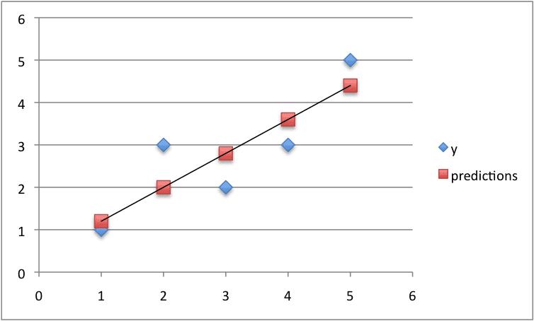
  Predictions For Small Contrived Dataset For Simple Linear Regression

  5. Predict Insurance

  We now know how to implement a simple linear regression model.

  Let’s apply it to the Swedish insurance dataset.

  This section assumes that you have downloaded the dataset to the file insurance.csv and it is available in the current working directory.

  We will add some convenience functions to the simple linear regression from the previous steps.

  Specifically a function to load the CSV file called load_csv(), a function to convert a loaded dataset to numbers called str_column_to_float(), a function to evaluate an algorithm using a train and test set called train_test_split() a function to calculate RMSE called rmse_metric() and a function to evaluate an algorithm called evaluate_algorithm().

  The complete example is listed below.

  A training dataset of 60% of the data is used to prepare the model and predictions are made on the remaining 40%.

  # Simple Linear Regression on the Swedish Insurance Dataset from random import seed from random import randrange from csv import reader from math import sqrt   # Load a CSV file def load_csv(filename): dataset = list() with open(filename, 'r') as file: csv_reader = reader(file) for row in csv_reader: if not row: continue dataset.append(row) return dataset   # Convert string column to float def str_column_to_float(dataset, column): for row in dataset: row[column] = float(row[column].strip())   # Split a dataset into a train and test set def train_test_split(dataset, split): train = list() train_size = split * len(dataset) dataset_copy = list(dataset) while len(train) < train_size: index = randrange(len(dataset_copy)) train.append(dataset_copy.pop(index)) return train, dataset_copy   # Calculate root mean squared error def rmse_metric(actual, predicted): sum_error = 0.0 for i in range(len(actual)): prediction_error = predicted[i] - actual[i] sum_error += (prediction_error ** 2) mean_error = sum_error / float(len(actual)) return sqrt(mean_error)   # Evaluate an algorithm using a train/test split def evaluate_algorithm(dataset, algorithm, split, *args): train, test = train_test_split(dataset, split) test_set = list() for row in test: row_copy = list(row) row_copy[-1] = None test_set.append(row_copy) predicted = algorithm(train, test_set, *args) actual = [row[-1] for row in test] rmse = rmse_metric(actual, predicted) return rmse   # Calculate the mean value of a list of numbers def mean(values): return sum(values) / float(len(values))   # Calculate covariance between x and y def covariance(x, mean_x, y, mean_y): covar = 0.0 for i in range(len(x)): covar += (x[i] - mean_x) * (y[i] - mean_y) return covar   # Calculate the variance of a list of numbers def variance(values, mean): return sum([(x-mean)**2 for x in values])   # Calculate coefficients def coefficients(dataset): x = [row[0] for row in dataset] y = [row[1] for row in dataset] x_mean, y_mean = mean(x), mean(y) b1 = covariance(x, x_mean, y, y_mean) / variance(x, x_mean) b0 = y_mean - b1 * x_mean return [b0, b1]   # Simple linear regression algorithm def simple_linear_regression(train, test): predictions = list() b0, b1 = coefficients(train) for row in test: yhat = b0 + b1 * row[0] predictions.append(yhat) return predictions   # Simple linear regression on insurance dataset seed(1) # load and prepare data filename = 'insurance.csv' dataset = load_csv(filename) for i in range(len(dataset[0])): str_column_to_float(dataset, i) # evaluate algorithm split = 0.6 rmse = evaluate_algorithm(dataset, simple_linear_regression, split) print('RMSE: %.3f' % (rmse))

  Running the algorithm prints the RMSE for the trained model on the training dataset.

  A score of about 33 (thousands of Kronor) was achieved, which is much better than the Zero Rule algorithm that achieves approximately 81 (thousands of Kronor) on the same problem.

  RMSE: 33.630

  Extensions

  The best extension to this tutorial is to try out the algorithm on more problems.

  Small datasets with just an input (x) and output (y) columns are popular for demonstration in statistical books and courses. Many of these datasets are available online.

  Seek out some more small datasets and make predictions using simple linear regression.

  Did you apply simple linear regression to another dataset?
  Share your experiences in the comments below.

  Review

  In this tutorial, you discovered how to implement the simple linear regression algorithm from scratch in Python.

  Specifically, you learned:

  • How to estimate statistics from a training dataset like mean, variance and covariance.
  • How to estimate model coefficients and use them to make predictions.
  • How to use simple linear regression to make predictions on a real dataset.