Ever looked at your data and thought something was missing or it’s hiding something from you? This is a deep dive guide on revealing those hidden connections and unknown relationships between the variables in your dataset.
Why should you care?
Machine learning algorithms like linear regression hate surprises.
It is essential to discover and quantify the degree to which variables in your dataset are dependent upon each other. This knowledge can help you better prepare your data to meet the expectations of machine learning algorithms, such as linear regression, whose performance will degrade with these interdependencies.
In this guide, you will discover that correlation is the statistical summary of the relationship between variables and how to calculate it for different types of variables and relationships.
After completing this tutorial, you will know:
- Covariance Matrix Magic: Summarize the linear bond between multiple variables.
- Pearson’s Power: Decode the linear ties between two variables.
- Spearman’s Insight: Unearth the unique monotonic rhythm between variables.
Kick-start your project with my new book Statistics for Machine Learning, including step-by-step tutorials and the Python source code files for all examples.
Let’s get started.
- Update May/2018: Updated description of the sign of the covariance (thanks Fulya).
- Update Nov/2023: Updated some wording for clarity and additional insights.
Tutorial Overview
This tutorial is divided into 5 parts; they are:
- What is Correlation?
- Test Dataset
- Covariance
- Pearson’s Correlation
- Spearman’s Correlation
What is Correlation?
Ever wondered how your data variables are linked to one another? Variables within a dataset can be related for lots of reasons.
For example:
- One variable could cause or depend on the values of another variable.
- One variable could be lightly associated with another variable.
- Two variables could depend on a third unknown variable.
All of these aspects of correlation and how data variables are dependent or can relate to one another get us thinking about their use. Correlation is very useful in data analysis and modelling to better understand the relationships between variables. The statistical relationship between two variables is referred to as their correlation.
A correlation could be presented in different ways:
- Positive Correlation: both variables change in the same direction.
- Neutral Correlation: No relationship in the change of the variables.
- Negative Correlation: variables change in opposite directions.
The performance of some algorithms can deteriorate if two or more variables are tightly related, called multicollinearity. An example is linear regression, where one of the offending correlated variables should be removed in order to improve the skill of the model.
We may also be interested in the correlation between input variables with the output variable in order to provide insight into which variables may or may not be relevant as input for developing a model.
The structure of the relationship may be known, e.g. it may be linear, or we may have no idea whether a relationship exists between two variables or what structure it may take. Depending on what is known about the relationship and the distribution of the variables, different correlation scores can be calculated.
In this tutorial guide, we will delve into a correlation score tailored for variables with a Gaussian distribution and a linear relationship. We will also explore another score that does not rely on a specific distribution and captures any monotonic (either increasing or decreasing) relationship.
Test Dataset
Before we go diving into correlation methods, let’s define a dataset we can use to test the methods.
We will generate 1,000 samples of two variables with a strong positive correlation. The first variable will be random numbers drawn from a Gaussian distribution with a mean of 100 and a standard deviation of 20. The second variable will be values from the first variable with Gaussian noise added with a mean of 50 and a standard deviation of 10.
We will use the randn() function to generate random Gaussian values with a mean of 0 and a standard deviation of 1, then multiply the results by our own standard deviation and add the mean to shift the values into the preferred range.
The pseudorandom number generator is seeded to ensure that we get the same sample of numbers each time the code is run.
1 2 3 4 5 6 7 8 9 10 11 12 13 14 15 16 17 | # generate related variables from numpy import mean from numpy import std from numpy.random import randn from numpy.random import seed from matplotlib import pyplot # seed random number generator seed(1) # prepare data data1 = 20 * randn(1000) + 100 data2 = data1 + (10 * randn(1000) + 50) # summarize print('data1: mean=%.3f stdv=%.3f' % (mean(data1), std(data1))) print('data2: mean=%.3f stdv=%.3f' % (mean(data2), std(data2))) # plot pyplot.scatter(data1, data2) pyplot.show() |
Executing the above code initially outputs the mean and standard deviation for both variables:
1 2 | data1: mean=100.776 stdv=19.620 data2: mean=151.050 stdv=22.358 |
A scatter plot of the two variables will be created. Because we contrived the dataset, we know there is a relationship between the two variables. This is clear when we review the generated scatter plot where we can see an increasing trend.
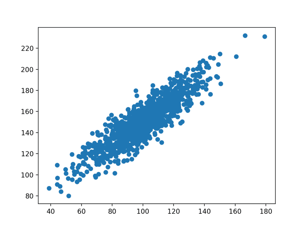
Scatter plot of the test correlation dataset
Before we look at calculating some correlation scores, it’s imperative to first comprehend a fundamental statistical concept known as covariance.
Covariance
You may have heard of linear relationships at school and also a lot in the world of data science. At the core of many statistical analyses is the concept of linear relationships between variables. This is a relationship that is consistently additive across the two data samples.
This relationship can be summarized between two variables, called the covariance. It is calculated as the average of the product between the values from each sample, where the values have been centred (by subtracting their respective means).
The calculation of the sample covariance is as follows:
1 | cov(X, Y) = (sum (x - mean(X)) * (y - mean(Y)) ) * 1/(n-1) |
The use of the mean in the calculation implies that each data should ideally adhere to a Gaussian or Gaussian-like distribution.
The covariance sign can be interpreted as whether the two variables change in the same direction (positive) or change in different directions (negative). The magnitude of the covariance is not easily interpreted. A covariance value of zero indicates that both variables are completely independent.
The cov() NumPy function can be used to calculate a covariance matrix between two or more variables.
1 | covariance = cov(data1, data2) |
The diagonal of the matrix contains the covariance between each variable and itself. The other values in the matrix represent the covariance between the two variables; in this case, the remaining two values are the same given that we are calculating the covariance for only two variables.
We can calculate the covariance matrix for the two variables in our test problem.
The complete example is listed below.
1 2 3 4 5 6 7 8 9 10 11 12 | # calculate the covariance between two variables from numpy.random import randn from numpy.random import seed from numpy import cov # seed random number generator seed(1) # prepare data data1 = 20 * randn(1000) + 100 data2 = data1 + (10 * randn(1000) + 50) # calculate covariance matrix covariance = cov(data1, data2) print(covariance) |
The covariance and covariance matrix are used widely within statistics and multivariate analysis to characterize the relationships between two or more variables.
Running the example calculates and prints the covariance matrix.
Because the dataset was contrived with each variable drawn from a Gaussian distribution and the variables linearly correlated, covariance is a reasonable method for describing the relationship.
The covariance between the two variables is 389.75. We can see that it is positive, suggesting the variables change in the same direction as we expect.
1 2 | [[385.33297729 389.7545618 ] [389.7545618 500.38006058]] |
A problem with covariance as a statistical tool alone is that it is challenging to interpret. This leads us to Pearson’s correlation coefficient next.
Pearson’s Correlation
Named after Karl Pearson, The Pearson correlation coefficient can be used to summarize the strength of the linear relationship between two data samples.
Pearson’s correlation coefficient is calculated by dividing the covariance of the two variables by the product of their respective standard deviations. It is the normalization of the covariance between the two variables to give an interpretable score.
1 | Pearson's correlation coefficient = covariance(X, Y) / (stdv(X) * stdv(Y)) |
The use of mean and standard deviation in the calculation suggests the need for the two data samples to have a Gaussian or Gaussian-like distribution.
The result of the calculation, the correlation coefficient can be interpreted to understand the relationship.
The coefficient returns a value between -1 and 1, symbolizing the full spectrum of correlation: from a complete negative correlation to a total positive correlation. A value of 0 means no correlation. The value must be interpreted, where often a value below -0.5 or above 0.5 indicates a notable correlation, and values below those values suggests a less notable correlation.
The pearsonr() SciPy function can be used to calculate the Pearson’s correlation coefficient between two data samples with the same length.
We can calculate the correlation between the two variables in our test problem.
The complete example is listed below.
1 2 3 4 5 6 7 8 9 10 11 12 | # calculate the Pearson's correlation between two variables from numpy.random import randn from numpy.random import seed from scipy.stats import pearsonr # seed random number generator seed(1) # prepare data data1 = 20 * randn(1000) + 100 data2 = data1 + (10 * randn(1000) + 50) # calculate Pearson's correlation corr, _ = pearsonr(data1, data2) print('Pearsons correlation: %.3f' % corr) |
Upon execution, Pearson’s correlation coefficient is determined and displayed. The evident positive correlation of 0.888 between the two variables is strong, as it surpasses the 0.5 threshold and approaches 1.0.
1 | Pearsons correlation: 0.888 |
Pearson’s correlation coefficient can be used to evaluate the relationship between more than two variables.
This can be done by calculating a matrix of the relationships between each pair of variables in the dataset. The result is a symmetric matrix called a correlation matrix with a value of 1.0 along the diagonal as each column always perfectly correlates with itself.
Spearman’s Correlation
While many data relationships can be linear, some may be nonlinear. These nonlinear relationships are stronger or weaker across the distribution of the variables. Further, the two variables being considered may have a non-Gaussian distribution.
Named after Charles Spearman, Spearman’s correlation coefficient can be used to summarize the strength between the two data samples. This test of relationship can also be used if there is a linear relationship between the variables but will have slightly less power (e.g. may result in lower coefficient scores).
As with the Pearson correlation coefficient, the scores are between -1 and 1 for perfectly negatively correlated variables and perfectly positively correlated respectively.
Instead of directly working with the data samples, it operates on the relative ranks of data values. This is a common approach used in non-parametric statistics, e.g. statistical methods where we do not assume a distribution of the data such as Gaussian.
1 | Spearman's correlation coefficient = covariance(rank(X), rank(Y)) / (stdv(rank(X)) * stdv(rank(Y))) |
A linear relationship between the variables is not assumed, although a monotonic relationship is assumed. This is a mathematical name for an increasing or decreasing relationship between the two variables.
If you are unsure of the distribution and possible relationships between two variables, the Spearman correlation coefficient is a good tool to use.
The spearmanr() SciPy function can be used to calculate the Spearman’s correlation coefficient between two data samples with the same length.
We can calculate the correlation between the two variables in our test problem.
The complete example is listed below.
1 2 3 4 5 6 7 8 9 10 11 12 | # calculate the spearmans's correlation between two variables from numpy.random import randn from numpy.random import seed from scipy.stats import spearmanr # seed random number generator seed(1) # prepare data data1 = 20 * randn(1000) + 100 data2 = data1 + (10 * randn(1000) + 50) # calculate spearman's correlation corr, _ = spearmanr(data1, data2) print('Spearmans correlation: %.3f' % corr) |
Running the example calculates and prints the Spearman’s correlation coefficient.
We know that the data is Gaussian and that the relationship between the variables is linear. Nevertheless, the nonparametric rank-based approach shows a strong correlation between the variables of 0.8.
1 | Spearmans correlation: 0.872 |
As with the Pearson’s correlation coefficient, the coefficient can be calculated pair-wise for each variable in a dataset to give a correlation matrix for review.
For more help with non-parametric correlation methods in Python, see:
Extensions
This section lists some ideas for extending the tutorial that you may wish to explore.
- Generate your own datasets with positive and negative relationships and calculate both correlation coefficients.
- Write functions to calculate Pearson or Spearman correlation matrices for a provided dataset.
- Load a standard machine learning dataset and calculate correlation coefficients between all pairs of real-valued variables.
If you explore any of these extensions, I’d love to know. Let me know your success stories in the comments below.
Further Reading
This section provides more resources on the topic if you are looking to go deeper.
Posts
- A Gentle Introduction to Expected Value, Variance, and Covariance with NumPy
- A Gentle Introduction to Autocorrelation and Partial Autocorrelation
API
- numpy.random.seed() API
- numpy.random.randn() API
- numpy.mean() API
- numpy.std() API
- matplotlib.pyplot.scatter() API
- numpy.cov() API
- scipy.stats.pearsonr() API
- scipy.stats.spearmanr() API
Articles
- Correlation and dependence on Wikipedia
- Covariance on Wikipedia
- Pearson correlation coefficient on Wikipedia
- Spearman’s rank correlation coefficient on Wikipedia
- Ranking on Wikipedia
Summary
In this tutorial, you discovered that correlation is the statistical summary of the relationship between variables and how to calculate it for different types variables and relationships.
Specifically, you learned:
- How to calculate a covariance matrix to summarize the linear relationship between two or more variables.
- How to calculate the Pearson’s correlation coefficient to summarize the linear relationship between two variables.
- How to calculate the Spearman’s correlation coefficient to summarize the monotonic relationship between two variables.
Do you have any questions?
Ask your questions in the comments below and I will do my best to answer.


No comments:
Post a Comment