Weight Regularization with LSTM Networks for Time Series Forecasting

 Long Short-Term Memory (LSTM) models are a recurrent neural network capable of learning sequences of observations.

This may make them a network well suited to time series forecasting.

An issue with LSTMs is that they can easily overfit training data, reducing their predictive skill.

Weight regularization is a technique for imposing constraints (such as L1 or L2) on the weights within LSTM nodes. This has the effect of reducing overfitting and improving model performance.

In this tutorial, you will discover how to use weight regularization with LSTM networks and design experiments to test for its effectiveness for time series forecasting.

After completing this tutorial, you will know:

• How to design a robust test harness for evaluating LSTM networks for time series forecasting.
• How to design, execute, and interpret the results from using bias weight regularization with LSTMs.
• How to design, execute, and interpret the results from using input and recurrent weight regularization with LSTMs.

  Tutorial Overview

  This tutorial is broken down into 6 parts. They are:

  1. Shampoo Sales Dataset
  2. Experimental Test Harness
  3. Bias Weight Regularization
  4. Input Weight Regularization
  5. Recurrent Weight Regularization
  6. Review of Results

  Environment

  This tutorial assumes you have a Python SciPy environment installed. You can use either Python 2 or 3 with this example.

  This tutorial assumes you have Keras v2.0 or higher installed with either the TensorFlow or Theano backend.

  This tutorial also assumes you have scikit-learn, Pandas, NumPy, and Matplotlib installed.Next, let’s take a look at a standard time series forecasting problem that we can use as context for this experiment.

  Shampoo Sales Dataset

  This dataset describes the monthly number of sales of shampoo over a 3-year period.

  The units are a sales count and there are 36 observations. The original dataset is credited to Makridakis, Wheelwright, and Hyndman (1998).

  • Download the dataset.

  The example below loads and creates a plot of the loaded dataset.

  # load and plot dataset from pandas import read_csv from pandas import datetime from matplotlib import pyplot # load dataset def parser(x): return datetime.strptime('190'+x, '%Y-%m') series = read_csv('shampoo-sales.csv', header=0, parse_dates=[0], index_col=0, squeeze=True, date_parser=parser) # summarize first few rows print(series.head()) # line plot series.plot() pyplot.show()

  Running the example loads the dataset as a Pandas Series and prints the first 5 rows.

  Month 1901-01-01 266.0 1901-02-01 145.9 1901-03-01 183.1 1901-04-01 119.3 1901-05-01 180.3 Name: Sales, dtype: float64

  A line plot of the series is then created showing a clear increasing trend.

  

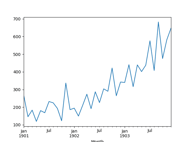
  Line Plot of Shampoo Sales Dataset

  Next, we will take a look at the model configuration and test harness used in the experiment.

  Experimental Test Harness

  This section describes the test harness used in this tutorial.

  Data Split

  We will split the Shampoo Sales dataset into two parts: a training and a test set.

  The first two years of data will be taken for the training dataset and the remaining one year of data will be used for the test set.

  Models will be developed using the training dataset and will make predictions on the test dataset.

  The persistence forecast (naive forecast) on the test dataset achieves an error of 136.761 monthly shampoo sales. This provides a lower acceptable bound of performance on the test set.

  Model Evaluation

  A rolling-forecast scenario will be used, also called walk-forward model validation.

  Each time step of the test dataset will be walked one at a time. A model will be used to make a forecast for the time step, then the actual expected value from the test set will be taken and made available to the model for the forecast on the next time step.

  This mimics a real-world scenario where new Shampoo Sales observations would be available each month and used in the forecasting of the following month.

  This will be simulated by the structure of the train and test datasets.

  All forecasts on the test dataset will be collected and an error score calculated to summarize the skill of the model. The root mean squared error (RMSE) will be used as it punishes large errors and results in a score that is in the same units as the forecast data, namely monthly shampoo sales.

  Data Preparation

  Before we can fit a model to the dataset, we must transform the data.

  The following three data transforms are performed on the dataset prior to fitting a model and making a forecast.

  1. Transform the time series data so that it is stationary. Specifically, a lag=1 differencing to remove the increasing trend in the data.
  2. Transform the time series into a supervised learning problem. Specifically, the organization of data into input and output patterns where the observation at the previous time step is used as an input to forecast the observation at the current timestep
  3. Transform the observations to have a specific scale. Specifically, to rescale the data to values between -1 and 1.

  These transforms are inverted on forecasts to return them into their original scale before calculating and error score.

  LSTM Model

  We will use a base stateful LSTM model with 1 neuron fit for 1000 epochs.

  Ideally a batch size of 1 would be used for walk-foward validation. We will assume walk-forward validation and predict the whole year for speed. As such we can use any batch size that is divisble by the number of samples, in this case we will use a value of 4.

  Ideally, more training epochs would be used (such as 1500), but this was truncated to 1000 to keep run times reasonable.

  The model will be fit using the efficient ADAM optimization algorithm and the mean squared error loss function.

  Experimental Runs

  Each experimental scenario will be run 30 times and the RMSE score on the test set will be recorded from the end each run.

  Let’s dive into the experiments.

  Baseline LSTM Model

  Let’s start-off with the baseline LSTM model.

  The baseline LSTM model for this problem has the following configuration:

  • Lag inputs: 1
  • Epochs: 1000
  • Units in LSTM hidden layer: 3
  • Batch Size: 4
  • Repeats: 3

  The complete code listing is provided below.

  This code listing will be used as the basis for all following experiments, with only the changes to this code provided in subsequent sections.

  from pandas import DataFrame from pandas import Series from pandas import concat from pandas import read_csv from pandas import datetime from sklearn.metrics import mean_squared_error from sklearn.preprocessing import MinMaxScaler from keras.models import Sequential from keras.layers import Dense from keras.layers import LSTM from keras.regularizers import L1L2 from math import sqrt import matplotlib # be able to save images on server matplotlib.use('Agg') from matplotlib import pyplot import numpy   # date-time parsing function for loading the dataset def parser(x): return datetime.strptime('190'+x, '%Y-%m')   # frame a sequence as a supervised learning problem def timeseries_to_supervised(data, lag=1): df = DataFrame(data) columns = [df.shift(i) for i in range(1, lag+1)] columns.append(df) df = concat(columns, axis=1) return df   # create a differenced series def difference(dataset, interval=1): diff = list() for i in range(interval, len(dataset)): value = dataset[i] - dataset[i - interval] diff.append(value) return Series(diff)   # invert differenced value def inverse_difference(history, yhat, interval=1): return yhat + history[-interval]   # scale train and test data to [-1, 1] def scale(train, test): # fit scaler scaler = MinMaxScaler(feature_range=(-1, 1)) scaler = scaler.fit(train) # transform train train = train.reshape(train.shape[0], train.shape[1]) train_scaled = scaler.transform(train) # transform test test = test.reshape(test.shape[0], test.shape[1]) test_scaled = scaler.transform(test) return scaler, train_scaled, test_scaled   # inverse scaling for a forecasted value def invert_scale(scaler, X, yhat): new_row = [x for x in X] + [yhat] array = numpy.array(new_row) array = array.reshape(1, len(array)) inverted = scaler.inverse_transform(array) return inverted[0, -1]   # fit an LSTM network to training data def fit_lstm(train, n_batch, nb_epoch, n_neurons): X, y = train[:, 0:-1], train[:, -1] X = X.reshape(X.shape[0], 1, X.shape[1]) model = Sequential() model.add(LSTM(n_neurons, batch_input_shape=(n_batch, X.shape[1], X.shape[2]), stateful=True)) model.add(Dense(1)) model.compile(loss='mean_squared_error', optimizer='adam') for i in range(nb_epoch): model.fit(X, y, epochs=1, batch_size=n_batch, verbose=0, shuffle=False) model.reset_states() return model   # run a repeated experiment def experiment(series, n_lag, n_repeats, n_epochs, n_batch, n_neurons): # transform data to be stationary raw_values = series.values diff_values = difference(raw_values, 1) # transform data to be supervised learning supervised = timeseries_to_supervised(diff_values, n_lag) supervised_values = supervised.values[n_lag:,:] # split data into train and test-sets train, test = supervised_values[0:-12], supervised_values[-12:] # transform the scale of the data scaler, train_scaled, test_scaled = scale(train, test) # run experiment error_scores = list() for r in range(n_repeats): # fit the model train_trimmed = train_scaled[2:, :] lstm_model = fit_lstm(train_trimmed, n_batch, n_epochs, n_neurons) # forecast test dataset test_reshaped = test_scaled[:,0:-1] test_reshaped = test_reshaped.reshape(len(test_reshaped), 1, 1) output = lstm_model.predict(test_reshaped, batch_size=n_batch) predictions = list() for i in range(len(output)): yhat = output[i,0] X = test_scaled[i, 0:-1] # invert scaling yhat = invert_scale(scaler, X, yhat) # invert differencing yhat = inverse_difference(raw_values, yhat, len(test_scaled)+1-i) # store forecast predictions.append(yhat) # report performance rmse = sqrt(mean_squared_error(raw_values[-12:], predictions)) print('%d) Test RMSE: %.3f' % (r+1, rmse)) error_scores.append(rmse) return error_scores   # configure the experiment def run(): # load dataset series = read_csv('shampoo-sales.csv', header=0, parse_dates=[0], index_col=0, squeeze=True, date_parser=parser) # configure the experiment n_lag = 1 n_repeats = 30 n_epochs = 1000 n_batch = 4 n_neurons = 3 # run the experiment results = DataFrame() results['results'] = experiment(series, n_lag, n_repeats, n_epochs, n_batch, n_neurons) # summarize results print(results.describe()) # save boxplot results.boxplot() pyplot.savefig('experiment_baseline.png')   # entry point run()

  Running the experiment prints summary statistics for the test RMSE for all repeats.

  Note: Your results may vary given the stochastic nature of the algorithm or evaluation procedure, or differences in numerical precision. Consider running the example a few times and compare the average outcome.

  We can see that on average, this model configuration achieves a test RMSE of about 92 monthly shampoo sales with a standard deviation of 5.

  results count   30.000000 mean    92.842537 std      5.748456 min     81.205979 25%     89.514367 50%     92.030003 75%     96.926145 max    105.247117

  A box and whisker plot is also created from the distribution of test RMSE results and saved to a file.

  The plot provides a clear depiction of the spread of the results, highlighting the middle 50% of values (the box) and the median (green line).

  

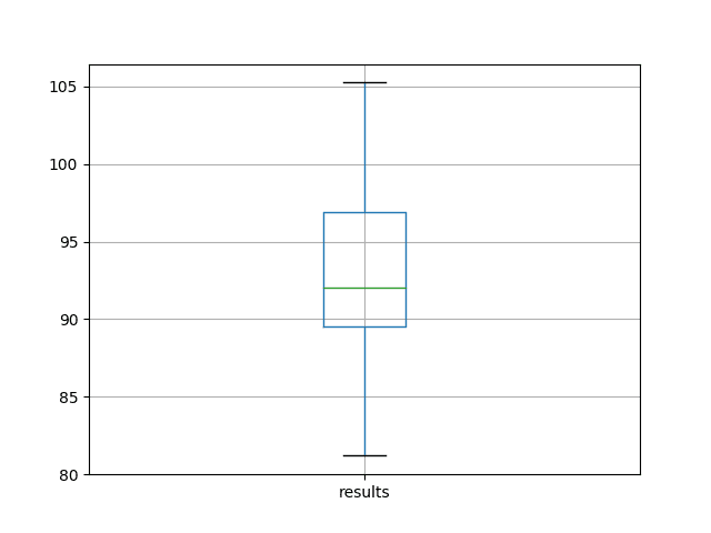
  Box and Whisker Plot of Baseline Performance on the Shampoo Sales Dataset

  Bias Weight Regularization

  Weight regularization can be applied to the bias connection within the LSTM nodes.

  In Keras, this is specified with a bias_regularizer argument when creating an LSTM layer. The regularizer is defined as an instance of the one of the L1, L2, or L1L2 classes.

  More details here:

  • Keras Usage of Regularizers

  In this experiment, we will compare L1, L2, and L1L2 with a default value of 0.01 against the baseline model. We can specify all configurations using the L1L2 class, as follows:

  • L1L2(0.0, 0.0) [e.g. baseline]
  • L1L2(0.01, 0.0) [e.g. L1]
  • L1L2(0.0, 0.01) [e.g. L2]
  • L1L2(0.01, 0.01) [e.g. L1L2 or elasticnet]

  Below lists the updated fit_lstm(), experiment(), and run() functions for using bias weight regularization with LSTMs.

  # fit an LSTM network to training data def fit_lstm(train, n_batch, nb_epoch, n_neurons, reg): X, y = train[:, 0:-1], train[:, -1] X = X.reshape(X.shape[0], 1, X.shape[1]) model = Sequential() model.add(LSTM(n_neurons, batch_input_shape=(n_batch, X.shape[1], X.shape[2]), stateful=True, bias_regularizer=reg)) model.add(Dense(1)) model.compile(loss='mean_squared_error', optimizer='adam') for i in range(nb_epoch): model.fit(X, y, epochs=1, batch_size=n_batch, verbose=0, shuffle=False) model.reset_states() return model   # run a repeated experiment def experiment(series, n_lag, n_repeats, n_epochs, n_batch, n_neurons, reg): # transform data to be stationary raw_values = series.values diff_values = difference(raw_values, 1) # transform data to be supervised learning supervised = timeseries_to_supervised(diff_values, n_lag) supervised_values = supervised.values[n_lag:,:] # split data into train and test-sets train, test = supervised_values[0:-12], supervised_values[-12:] # transform the scale of the data scaler, train_scaled, test_scaled = scale(train, test) # run experiment error_scores = list() for r in range(n_repeats): # fit the model train_trimmed = train_scaled[2:, :] lstm_model = fit_lstm(train_trimmed, n_batch, n_epochs, n_neurons, reg) # forecast test dataset test_reshaped = test_scaled[:,0:-1] test_reshaped = test_reshaped.reshape(len(test_reshaped), 1, 1) output = lstm_model.predict(test_reshaped, batch_size=n_batch) predictions = list() for i in range(len(output)): yhat = output[i,0] X = test_scaled[i, 0:-1] # invert scaling yhat = invert_scale(scaler, X, yhat) # invert differencing yhat = inverse_difference(raw_values, yhat, len(test_scaled)+1-i) # store forecast predictions.append(yhat) # report performance rmse = sqrt(mean_squared_error(raw_values[-12:], predictions)) print('%d) Test RMSE: %.3f' % (r+1, rmse)) error_scores.append(rmse) return error_scores   # configure the experiment def run(): # load dataset series = read_csv('shampoo-sales.csv', header=0, parse_dates=[0], index_col=0, squeeze=True, date_parser=parser) # configure the experiment n_lag = 1 n_repeats = 30 n_epochs = 1000 n_batch = 4 n_neurons = 3 regularizers = [L1L2(l1=0.0, l2=0.0), L1L2(l1=0.01, l2=0.0), L1L2(l1=0.0, l2=0.01), L1L2(l1=0.01, l2=0.01)] # run the experiment results = DataFrame() for reg in regularizers: name = ('l1 %.2f,l2 %.2f' % (reg.l1, reg.l2)) results[name] = experiment(series, n_lag, n_repeats, n_epochs, n_batch, n_neurons, reg) # summarize results print(results.describe()) # save boxplot results.boxplot() pyplot.savefig('experiment_reg_bias.png')

  Running this experiment prints descriptive statistics for each evaluated configuration.

  Note: Your results may vary given the stochastic nature of the algorithm or evaluation procedure, or differences in numerical precision. Consider running the example a few times and compare the average outcome.

  The results suggest that on average, the default of no bias regularization results in better performance compared to all of the other configurations considered.

  l1 0.00,l2 0.00  l1 0.01,l2 0.00  l1 0.00,l2 0.01  l1 0.01,l2 0.01 count        30.000000        30.000000        30.000000        30.000000 mean         92.821489        95.520003        93.285389        92.901021 std           4.894166         3.637022         3.906112         5.082358 min          81.394504        89.477398        82.994480        78.729224 25%          89.356330        93.017723        90.907343        91.210105 50%          92.822871        95.502700        93.837562        94.525965 75%          95.899939        98.195980        95.426270        96.882378 max         101.194678       101.750900       100.650130        97.766301

  A box and whisker plot is also created to compare the distributions of results for each configuration.

  The plot shows that all configurations have about the same spread and that the addition of bias regularization uniformly was not helpful on this problem.

  

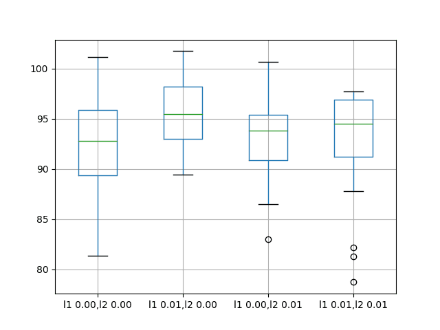
  Box and Whisker Plots of Bias Weight Regularization Performance on the Shampoo Sales Dataset

  Input Weight Regularization

  We can also apply regularization to input connections on each LSTM unit.

  In Keras, this is achieved by setting the kernel_regularizer argument to a regularizer class.

  We will test the same regularizer configurations as were used in the previous section, specifically:

  • L1L2(0.0, 0.0) [e.g. baseline]
  • L1L2(0.01, 0.0) [e.g. L1]
  • L1L2(0.0, 0.01) [e.g. L2]
  • L1L2(0.01, 0.01) [e.g. L1L2 or elasticnet]

  Below lists the updated fit_lstm(), experiment(), and run() functions for using bias weight regularization with LSTMs.

  # fit an LSTM network to training data def fit_lstm(train, n_batch, nb_epoch, n_neurons, reg): X, y = train[:, 0:-1], train[:, -1] X = X.reshape(X.shape[0], 1, X.shape[1]) model = Sequential() model.add(LSTM(n_neurons, batch_input_shape=(n_batch, X.shape[1], X.shape[2]), stateful=True, kernel_regularizer=reg)) model.add(Dense(1)) model.compile(loss='mean_squared_error', optimizer='adam') for i in range(nb_epoch): model.fit(X, y, epochs=1, batch_size=n_batch, verbose=0, shuffle=False) model.reset_states() return model   # run a repeated experiment def experiment(series, n_lag, n_repeats, n_epochs, n_batch, n_neurons, reg): # transform data to be stationary raw_values = series.values diff_values = difference(raw_values, 1) # transform data to be supervised learning supervised = timeseries_to_supervised(diff_values, n_lag) supervised_values = supervised.values[n_lag:,:] # split data into train and test-sets train, test = supervised_values[0:-12], supervised_values[-12:] # transform the scale of the data scaler, train_scaled, test_scaled = scale(train, test) # run experiment error_scores = list() for r in range(n_repeats): # fit the model train_trimmed = train_scaled[2:, :] lstm_model = fit_lstm(train_trimmed, n_batch, n_epochs, n_neurons, reg) # forecast test dataset test_reshaped = test_scaled[:,0:-1] test_reshaped = test_reshaped.reshape(len(test_reshaped), 1, 1) output = lstm_model.predict(test_reshaped, batch_size=n_batch) predictions = list() for i in range(len(output)): yhat = output[i,0] X = test_scaled[i, 0:-1] # invert scaling yhat = invert_scale(scaler, X, yhat) # invert differencing yhat = inverse_difference(raw_values, yhat, len(test_scaled)+1-i) # store forecast predictions.append(yhat) # report performance rmse = sqrt(mean_squared_error(raw_values[-12:], predictions)) print('%d) Test RMSE: %.3f' % (r+1, rmse)) error_scores.append(rmse) return error_scores   # configure the experiment def run(): # load dataset series = read_csv('shampoo-sales.csv', header=0, parse_dates=[0], index_col=0, squeeze=True, date_parser=parser) # configure the experiment n_lag = 1 n_repeats = 30 n_epochs = 1000 n_batch = 4 n_neurons = 3 regularizers = [L1L2(l1=0.0, l2=0.0), L1L2(l1=0.01, l2=0.0), L1L2(l1=0.0, l2=0.01), L1L2(l1=0.01, l2=0.01)] # run the experiment results = DataFrame() for reg in regularizers: name = ('l1 %.2f,l2 %.2f' % (reg.l1, reg.l2)) results[name] = experiment(series, n_lag, n_repeats, n_epochs, n_batch, n_neurons, reg) # summarize results print(results.describe()) # save boxplot results.boxplot() pyplot.savefig('experiment_reg_input.png')

  Running this experiment prints descriptive statistics for each evaluated configuration.

  Note: Your results may vary given the stochastic nature of the algorithm or evaluation procedure, or differences in numerical precision. Consider running the example a few times and compare the average outcome.

  The results suggest that adding weight regularization to input connections does offer benefit across the board on this setup.

  We can see that the test RMSE is approximately 10 units lower for all configurations with perhaps more benefit when both L1 and L2 are combined into an elasticnet type constraint.

  l1 0.00,l2 0.00  l1 0.01,l2 0.00  l1 0.00,l2 0.01  l1 0.01,l2 0.01 count        30.000000        30.000000        30.000000        30.000000 mean         91.640028        82.118980        82.137198        80.471685 std           6.086401         4.116072         3.378984         2.212213 min          80.392310        75.705210        76.005173        76.550909 25%          88.025135        79.237822        79.698162        78.780802 50%          91.843761        81.235433        81.463882        80.283913 75%          94.860117        85.510177        84.563980        82.443390 max         105.820586        94.210503        90.823454        85.243135

  A box and whisker plot is also created to compare the distributions of results for each configuration.

  The plot shows the general lower distribution of error for input regularization. The results also suggest a tighter spread of results with regularization that may be more pronounced with the L1L2 configuration that achieved the better results.

  This is an encouraging finding, suggesting that additional experiments with different L1L2 values for input regularization would be well worth investigating.

  

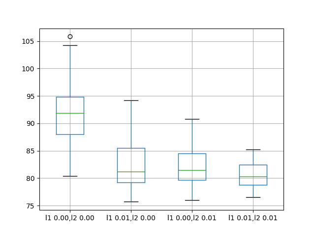
  Box and Whisker Plots of Input Weight Regularization Performance on the Shampoo Sales Dataset

  Recurrent Weight Regularization

  Finally, we can also apply regularization to recurrent connections on each LSTM unit.

  In Keras, this is achieved by setting the recurrent_regularizer argument to a regularizer class.

  We will test the same regularizer configurations as were used in the previous section, specifically:

  • L1L2(0.0, 0.0) [e.g. baseline]
  • L1L2(0.01, 0.0) [e.g. L1]
  • L1L2(0.0, 0.01) [e.g. L2]
  • L1L2(0.01, 0.01) [e.g. L1L2 or elasticnet]

  Below lists the updated fit_lstm(), experiment(), and run() functions for using bias weight regularization with LSTMs.

  # fit an LSTM network to training data def fit_lstm(train, n_batch, nb_epoch, n_neurons, reg): X, y = train[:, 0:-1], train[:, -1] X = X.reshape(X.shape[0], 1, X.shape[1]) model = Sequential() model.add(LSTM(n_neurons, batch_input_shape=(n_batch, X.shape[1], X.shape[2]), stateful=True, recurrent_regularizer=reg)) model.add(Dense(1)) model.compile(loss='mean_squared_error', optimizer='adam') for i in range(nb_epoch): model.fit(X, y, epochs=1, batch_size=n_batch, verbose=0, shuffle=False) model.reset_states() return model   # run a repeated experiment def experiment(series, n_lag, n_repeats, n_epochs, n_batch, n_neurons, reg): # transform data to be stationary raw_values = series.values diff_values = difference(raw_values, 1) # transform data to be supervised learning supervised = timeseries_to_supervised(diff_values, n_lag) supervised_values = supervised.values[n_lag:,:] # split data into train and test-sets train, test = supervised_values[0:-12], supervised_values[-12:] # transform the scale of the data scaler, train_scaled, test_scaled = scale(train, test) # run experiment error_scores = list() for r in range(n_repeats): # fit the model train_trimmed = train_scaled[2:, :] lstm_model = fit_lstm(train_trimmed, n_batch, n_epochs, n_neurons, reg) # forecast test dataset test_reshaped = test_scaled[:,0:-1] test_reshaped = test_reshaped.reshape(len(test_reshaped), 1, 1) output = lstm_model.predict(test_reshaped, batch_size=n_batch) predictions = list() for i in range(len(output)): yhat = output[i,0] X = test_scaled[i, 0:-1] # invert scaling yhat = invert_scale(scaler, X, yhat) # invert differencing yhat = inverse_difference(raw_values, yhat, len(test_scaled)+1-i) # store forecast predictions.append(yhat) # report performance rmse = sqrt(mean_squared_error(raw_values[-12:], predictions)) print('%d) Test RMSE: %.3f' % (r+1, rmse)) error_scores.append(rmse) return error_scores   # configure the experiment def run(): # load dataset series = read_csv('shampoo-sales.csv', header=0, parse_dates=[0], index_col=0, squeeze=True, date_parser=parser) # configure the experiment n_lag = 1 n_repeats = 30 n_epochs = 1000 n_batch = 4 n_neurons = 3 regularizers = [L1L2(l1=0.0, l2=0.0), L1L2(l1=0.01, l2=0.0), L1L2(l1=0.0, l2=0.01), L1L2(l1=0.01, l2=0.01)] # run the experiment results = DataFrame() for reg in regularizers: name = ('l1 %.2f,l2 %.2f' % (reg.l1, reg.l2)) results[name] = experiment(series, n_lag, n_repeats, n_epochs, n_batch, n_neurons, reg) # summarize results print(results.describe()) # save boxplot results.boxplot() pyplot.savefig('experiment_reg_recurrent.png')

  Running this experiment prints descriptive statistics for each evaluated configuration.

  Note: Your results may vary given the stochastic nature of the algorithm or evaluation procedure, or differences in numerical precision. Consider running the example a few times and compare the average outcome.

  The results suggest no obvious benefit from using regularization on the recurrent connection with LSTMs on this problem.

  The mean performance of all variations tried resulted in worse performance than the baseline model.

  l1 0.00,l2 0.00  l1 0.01,l2 0.00  l1 0.00,l2 0.01  l1 0.01,l2 0.01 count        30.000000        30.000000        30.000000        30.000000 mean         92.918797       100.675386       101.302169        96.820026 std           7.172764         3.866547         5.228815         3.966710 min          72.967841        93.789854        91.063592        89.367600 25%          90.311185        98.014045        98.222732        94.787647 50%          92.327824       100.546756       101.903350        95.727549 75%          95.989761       103.491192       104.918266        98.240613 max         110.529422       108.788604       110.712064       111.185747

  A box and whisker plot is also created to compare the distributions of results for each configuration.

  The plot shows the same story as the summary statistics, suggesting little benefit from using recurrent weight regularization.

  

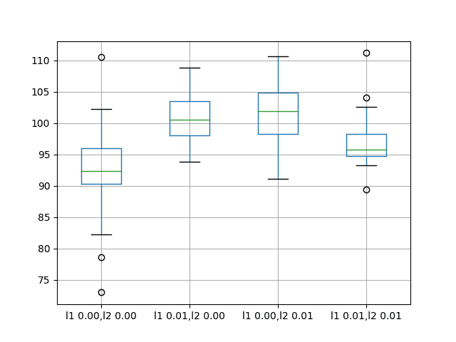
  Box and Whisker Plots of Recurrent Weight Regularization Performance on the Shampoo Sales Dataset

  Extensions

  This section lists ideas for follow-up experiments to extend the work in this tutorial.

  • Input Weight Regularization. The experimental results for input weight regularization on this problem showed great promise of listing performance. This could be investigated further by perhaps grid searching different L1 and L2 values to find an optimal configuration.
  • Behavior Dynamics. The dynamic behavior of each weight regularization scheme could be investigated by plotting train and test RMSE over training epochs to get an idea of weight regularization on overfitting or underfitting behavior patterns.
  • Combine Regularization. Experiments could be designed to explore the effect of combining different weight regularization schemes.
  • Activation Regularization. Keras also supports activation regularization, and this could be another avenue to explore imposing constraints on the LSTM and reduce overfitting.

  Summary

  In this tutorial, you discovered how to use weight regularization with LSTMs for time series forecasting.

  Specifically, you learned:

  • How to design a robust test harness for evaluating LSTM networks for time series forecasting.
  • How to configure bias weight regularization on LSTMs for time series forecasting.
  • How to configure input and recurrent weight regularization on LSTMs for time series forecasting.

  Do you have any questions about using weight regularization with LSTM networks?
  Ask your questions in the comments below and I will do my best to answer.