How to evaluate a multi-step time series forecast.Tutorial Overview
This tutorial is broken down into 4 parts; they are:
- Shampoo Sales Dataset
- Data Preparation and Model Evaluation
- Persistence Model
- Multi-Step LSTM
Environment
This tutorial assumes you have a Python SciPy environment installed. You can use either Python 2 or 3 with this example.
This tutorial assumes you have Keras v2.0 or higher installed with either the TensorFlow or Theano backend.
This tutorial also assumes you have scikit-learn, Pandas, NumPy, and Matplotlib installed.
If you need help setting up your Python environment, see this post:
Next, let’s take a look at a standard time series forecasting problem that we can use as context for this experiment.
Need help with Deep Learning for Time Series?
Take my free 7-day email crash course now (with sample code).
Click to sign-up and also get a free PDF Ebook version of the course.
Shampoo Sales Dataset
This dataset describes the monthly number of sales of shampoo over a 3-year period.
The units are a sales count and there are 36 observations. The
original dataset is credited to Makridakis, Wheelwright, and Hyndman
(1998).
The example below loads and creates a plot of the loaded dataset.
# load and plot dataset from pandas import read_csv from pandas import datetime from matplotlib import pyplot # load dataset def parser(x): return datetime.strptime('190'+x, '%Y-%m') series = read_csv('shampoo-sales.csv', header=0, parse_dates=[0], index_col=0, squeeze=True, date_parser=parser) # summarize first few rows print(series.head()) # line plot series.plot() pyplot.show() |
Running the example loads the dataset as a Pandas Series and prints the first 5 rows.
Month 1901-01-01 266.0 1901-02-01 145.9 1901-03-01 183.1 1901-04-01 119.3 1901-05-01 180.3 Name: Sales, dtype: float64 |
A line plot of the series is then created showing a clear increasing trend.
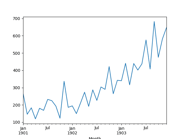
Line Plot of Shampoo Sales Dataset
Next, we will take a look at the model configuration and test harness used in the experiment.
Data Preparation and Model Evaluation
This section describes data preparation and model evaluation used in this tutorial
Data Split
We will split the Shampoo Sales dataset into two parts: a training and a test set.
The first two years of data will be taken for the training dataset
and the remaining one year of data will be used for the test set.
Models will be developed using the training dataset and will make predictions on the test dataset.
For reference, the last 12 months of observations are as follows:
"3-01",339.7 "3-02",440.4 "3-03",315.9 "3-04",439.3 "3-05",401.3 "3-06",437.4 "3-07",575.5 "3-08",407.6 "3-09",682.0 "3-10",475.3 "3-11",581.3 "3-12",646.9 |
Multi-Step Forecast
We will contrive a multi-step forecast.
For a given month in the final 12 months of the dataset, we will be required to make a 3-month forecast.
That is given historical observations (t-1, t-2, … t-n) forecast t, t+1 and t+2.
Specifically, from December in year 2, we must forecast January,
February and March. From January, we must forecast February, March and
April. All the way to an October, November, December forecast from
September in year 3.
A total of 10 3-month forecasts are required, as follows:
Dec, Jan, Feb, Mar Jan, Feb, Mar, Apr Feb, Mar, Apr, May Mar, Apr, May, Jun Apr, May, Jun, Jul May, Jun, Jul, Aug Jun, Jul, Aug, Sep Jul, Aug, Sep, Oct Aug, Sep, Oct, Nov Sep, Oct, Nov, Dec |
Model Evaluation
A rolling-forecast scenario will be used, also called walk-forward model validation.
Each time step of the test dataset will be walked one at a time. A
model will be used to make a forecast for the time step, then the actual
expected value for the next month from the test set will be taken and
made available to the model for the forecast on the next time step.
This mimics a real-world scenario where new Shampoo Sales
observations would be available each month and used in the forecasting
of the following month.
This will be simulated by the structure of the train and test datasets.
All forecasts on the test dataset will be collected and an error
score calculated to summarize the skill of the model for each of the
forecast time steps. The root mean squared error (RMSE) will be used as
it punishes large errors and results in a score that is in the same
units as the forecast data, namely monthly shampoo sales.
Persistence Model
A good baseline for time series forecasting is the persistence model.
This is a forecasting model where the last observation is persisted
forward. Because of its simplicity, it is often called the naive
forecast.
You can learn more about the persistence model for time series forecasting in the post:
Prepare Data
The first step is to transform the data from a series into a supervised learning problem.
That is to go from a list of numbers to a list of input and output
patterns. We can achieve this using a pre-prepared function called series_to_supervised().
For more on this function, see the post:
The function is listed below.
# convert time series into supervised learning problem def series_to_supervised(data, n_in=1, n_out=1, dropnan=True): n_vars = 1 if type(data) is list else data.shape[1] df = DataFrame(data) cols, names = list(), list() # input sequence (t-n, ... t-1) for i in range(n_in, 0, -1): cols.append(df.shift(i)) names += [('var%d(t-%d)' % (j+1, i)) for j in range(n_vars)] # forecast sequence (t, t+1, ... t+n) for i in range(0, n_out): cols.append(df.shift(-i)) if i == 0: names += [('var%d(t)' % (j+1)) for j in range(n_vars)] else: names += [('var%d(t+%d)' % (j+1, i)) for j in range(n_vars)] # put it all together agg = concat(cols, axis=1) agg.columns = names # drop rows with NaN values if dropnan: agg.dropna(inplace=True) return agg |
The function can be called by passing in the loaded series values an n_in value of 1 and an n_out value of 3; for example:
supervised = series_to_supervised(raw_values, 1, 3) |
Next, we can split the supervised learning dataset into training and test sets.
We know that in this form, the last 10 rows contain data for the
final year. These rows comprise the test set and the rest of the data
makes up the training dataset.
We can put all of this together in a new function that takes the
loaded series and some parameters and returns a train and test set ready
for modeling.
# transform series into train and test sets for supervised learning def prepare_data(series, n_test, n_lag, n_seq): # extract raw values raw_values = series.values raw_values = raw_values.reshape(len(raw_values), 1) # transform into supervised learning problem X, y supervised = series_to_supervised(raw_values, n_lag, n_seq) supervised_values = supervised.values # split into train and test sets train, test = supervised_values[0:-n_test], supervised_values[-n_test:] return train, test |
We can test this with the Shampoo dataset. The complete example is listed below.
from pandas import DataFrame from pandas import concat from pandas import read_csv from pandas import datetime # date-time parsing function for loading the dataset def parser(x): return datetime.strptime('190'+x, '%Y-%m') # convert time series into supervised learning problem def series_to_supervised(data, n_in=1, n_out=1, dropnan=True): n_vars = 1 if type(data) is list else data.shape[1] df = DataFrame(data) cols, names = list(), list() # input sequence (t-n, ... t-1) for i in range(n_in, 0, -1): cols.append(df.shift(i)) names += [('var%d(t-%d)' % (j+1, i)) for j in range(n_vars)] # forecast sequence (t, t+1, ... t+n) for i in range(0, n_out): cols.append(df.shift(-i)) if i == 0: names += [('var%d(t)' % (j+1)) for j in range(n_vars)] else: names += [('var%d(t+%d)' % (j+1, i)) for j in range(n_vars)] # put it all together agg = concat(cols, axis=1) agg.columns = names # drop rows with NaN values if dropnan: agg.dropna(inplace=True) return agg # transform series into train and test sets for supervised learning def prepare_data(series, n_test, n_lag, n_seq): # extract raw values raw_values = series.values raw_values = raw_values.reshape(len(raw_values), 1) # transform into supervised learning problem X, y supervised = series_to_supervised(raw_values, n_lag, n_seq) supervised_values = supervised.values # split into train and test sets train, test = supervised_values[0:-n_test], supervised_values[-n_test:] return train, test # load dataset series = read_csv('shampoo-sales.csv', header=0, parse_dates=[0], index_col=0, squeeze=True, date_parser=parser) # configure n_lag = 1 n_seq = 3 n_test = 10 # prepare data train, test = prepare_data(series, n_test, n_lag, n_seq) print(test) print('Train: %s, Test: %s' % (train.shape, test.shape)) |
Running the example first prints the entire test dataset, which
is the last 10 rows. The shape and size of the train test datasets is
also printed.
[[ 342.3 339.7 440.4 315.9] [ 339.7 440.4 315.9 439.3] [ 440.4 315.9 439.3 401.3] [ 315.9 439.3 401.3 437.4] [ 439.3 401.3 437.4 575.5] [ 401.3 437.4 575.5 407.6] [ 437.4 575.5 407.6 682. ] [ 575.5 407.6 682. 475.3] [ 407.6 682. 475.3 581.3] [ 682. 475.3 581.3 646.9]] Train: (23, 4), Test: (10, 4) |
We can see the single input value (first column) on the first
row of the test dataset matches the observation in the shampoo-sales for
December in the 2nd year:
We can also see that each row contains 4 columns for the 1 input and 3 output values in each observation.
Make Forecasts
The next step is to make persistence forecasts.
We can implement the persistence forecast easily in a function named persistence()
that takes the last observation and the number of forecast steps to
persist. This function returns an array containing the forecast.
# make a persistence forecast def persistence(last_ob, n_seq): return [last_ob for i in range(n_seq)] |
We can then call this function for each time step in the test dataset from December in year 2 to September in year 3.
Below is a function make_forecasts() that does this and takes the train, test, and configuration for the dataset as arguments and returns a list of forecasts.
# evaluate the persistence model def make_forecasts(train, test, n_lag, n_seq): forecasts = list() for i in range(len(test)): X, y = test[i, 0:n_lag], test[i, n_lag:] # make forecast forecast = persistence(X[-1], n_seq) # store the forecast forecasts.append(forecast) return forecasts |
We can call this function as follows:
forecasts = make_forecasts(train, test, 1, 3) |
Evaluate Forecasts
The final step is to evaluate the forecasts.
We can do that by calculating the RMSE for each time step of the
multi-step forecast, in this case giving us 3 RMSE scores. The function
below, evaluate_forecasts(), calculates and prints the RMSE for each forecasted time step.
# evaluate the RMSE for each forecast time step def evaluate_forecasts(test, forecasts, n_lag, n_seq): for i in range(n_seq): actual = test[:,(n_lag+i)] predicted = [forecast[i] for forecast in forecasts] rmse = sqrt(mean_squared_error(actual, predicted)) print('t+%d RMSE: %f' % ((i+1), rmse)) |
We can call it as follows:
evaluate_forecasts(test, forecasts, 1, 3) |
It is also helpful to plot the forecasts in the context of the
original dataset to get an idea of how the RMSE scores relate to the
problem in context.
We can first plot the entire Shampoo dataset, then plot each forecast as a red line. The function plot_forecasts() below will create and show this plot.
# plot the forecasts in the context of the original dataset def plot_forecasts(series, forecasts, n_test): # plot the entire dataset in blue pyplot.plot(series.values) # plot the forecasts in red for i in range(len(forecasts)): off_s = len(series) - n_test + i off_e = off_s + len(forecasts[i]) xaxis = [x for x in range(off_s, off_e)] pyplot.plot(xaxis, forecasts[i], color='red') # show the plot pyplot.show() |
We can call the function as follows. Note that the number of
observations held back on the test set is 12 for the 12 months, as
opposed to 10 for the 10 supervised learning input/output patterns as
was used above.
# plot forecasts plot_forecasts(series, forecasts, 12) |
We can make the plot better by connecting the persisted forecast to the actual persisted value in the original dataset.
This will require adding the last observed value to the front of the forecast. Below is an updated version of the plot_forecasts() function with this improvement.
# plot the forecasts in the context of the original dataset def plot_forecasts(series, forecasts, n_test): # plot the entire dataset in blue pyplot.plot(series.values) # plot the forecasts in red for i in range(len(forecasts)): off_s = len(series) - 12 + i - 1 off_e = off_s + len(forecasts[i]) + 1 xaxis = [x for x in range(off_s, off_e)] yaxis = [series.values[off_s]] + forecasts[i] pyplot.plot(xaxis, yaxis, color='red') # show the plot pyplot.show() |
Complete Example
We can put all of these pieces together.
The complete code example for the multi-step persistence forecast is listed below.
from pandas import DataFrame from pandas import concat from pandas import read_csv from pandas import datetime from sklearn.metrics import mean_squared_error from math import sqrt from matplotlib import pyplot # date-time parsing function for loading the dataset def parser(x): return datetime.strptime('190'+x, '%Y-%m') # convert time series into supervised learning problem def series_to_supervised(data, n_in=1, n_out=1, dropnan=True): n_vars = 1 if type(data) is list else data.shape[1] df = DataFrame(data) cols, names = list(), list() # input sequence (t-n, ... t-1) for i in range(n_in, 0, -1): cols.append(df.shift(i)) names += [('var%d(t-%d)' % (j+1, i)) for j in range(n_vars)] # forecast sequence (t, t+1, ... t+n) for i in range(0, n_out): cols.append(df.shift(-i)) if i == 0: names += [('var%d(t)' % (j+1)) for j in range(n_vars)] else: names += [('var%d(t+%d)' % (j+1, i)) for j in range(n_vars)] # put it all together agg = concat(cols, axis=1) agg.columns = names # drop rows with NaN values if dropnan: agg.dropna(inplace=True) return agg # transform series into train and test sets for supervised learning def prepare_data(series, n_test, n_lag, n_seq): # extract raw values raw_values = series.values raw_values = raw_values.reshape(len(raw_values), 1) # transform into supervised learning problem X, y supervised = series_to_supervised(raw_values, n_lag, n_seq) supervised_values = supervised.values # split into train and test sets train, test = supervised_values[0:-n_test], supervised_values[-n_test:] return train, test # make a persistence forecast def persistence(last_ob, n_seq): return [last_ob for i in range(n_seq)] # evaluate the persistence model def make_forecasts(train, test, n_lag, n_seq): forecasts = list() for i in range(len(test)): X, y = test[i, 0:n_lag], test[i, n_lag:] # make forecast forecast = persistence(X[-1], n_seq) # store the forecast forecasts.append(forecast) return forecasts # evaluate the RMSE for each forecast time step def evaluate_forecasts(test, forecasts, n_lag, n_seq): for i in range(n_seq): actual = test[:,(n_lag+i)] predicted = [forecast[i] for forecast in forecasts] rmse = sqrt(mean_squared_error(actual, predicted)) print('t+%d RMSE: %f' % ((i+1), rmse)) # plot the forecasts in the context of the original dataset def plot_forecasts(series, forecasts, n_test): # plot the entire dataset in blue pyplot.plot(series.values) # plot the forecasts in red for i in range(len(forecasts)): off_s = len(series) - n_test + i - 1 off_e = off_s + len(forecasts[i]) + 1 xaxis = [x for x in range(off_s, off_e)] yaxis = [series.values[off_s]] + forecasts[i] pyplot.plot(xaxis, yaxis, color='red') # show the plot pyplot.show() # load dataset series = read_csv('shampoo-sales.csv', header=0, parse_dates=[0], index_col=0, squeeze=True, date_parser=parser) # configure n_lag = 1 n_seq = 3 n_test = 10 # prepare data train, test = prepare_data(series, n_test, n_lag, n_seq) # make forecasts forecasts = make_forecasts(train, test, n_lag, n_seq) # evaluate forecasts evaluate_forecasts(test, forecasts, n_lag, n_seq) # plot forecasts plot_forecasts(series, forecasts, n_test+2) |
Running the example first prints the RMSE for each of the forecasted time steps.
Note: Your results may vary
given the stochastic nature of the algorithm or evaluation procedure,
or differences in numerical precision. Consider running the example a
few times and compare the average outcome.
This gives us a baseline of performance on each time step that we would expect the LSTM to outperform.
t+1 RMSE: 144.535304 t+2 RMSE: 86.479905 t+3 RMSE: 121.149168 |
The plot of the original time series with the multi-step
persistence forecasts is also created. The lines connect to the
appropriate input value for each forecast.
This context shows how naive the persistence forecasts actually are.
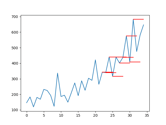
Line Plot of Shampoo Sales Dataset with Multi-Step Persistence Forecasts
Multi-Step LSTM Network
In this section, we will use the persistence example as a starting
point and look at the changes needed to fit an LSTM to the training data
and make multi-step forecasts for the test dataset.
Prepare Data
The data must be prepared before we can use it to train an LSTM.
Specifically, two additional changes are required:
- Stationary. The data shows an increasing trend that must be removed by differencing.
- Scale. The scale of the data must be reduced to values between -1 and 1, the activation function of the LSTM units.
We can introduce a function to make the data stationary called difference(). This will transform the series of values into a series of differences, a simpler representation to work with.
# create a differenced series def difference(dataset, interval=1): diff = list() for i in range(interval, len(dataset)): value = dataset[i] - dataset[i - interval] diff.append(value) return Series(diff) |
We can use the MinMaxScaler from the sklearn library to scale the data.
Putting this together, we can update the prepare_data()
function to first difference the data and rescale it, then perform the
transform into a supervised learning problem and train test sets as we
did before with the persistence example.
The function now returns a scaler in addition to the train and test datasets.
# transform series into train and test sets for supervised learning def prepare_data(series, n_test, n_lag, n_seq): # extract raw values raw_values = series.values # transform data to be stationary diff_series = difference(raw_values, 1) diff_values = diff_series.values diff_values = diff_values.reshape(len(diff_values), 1) # rescale values to -1, 1 scaler = MinMaxScaler(feature_range=(-1, 1)) scaled_values = scaler.fit_transform(diff_values) scaled_values = scaled_values.reshape(len(scaled_values), 1) # transform into supervised learning problem X, y supervised = series_to_supervised(scaled_values, n_lag, n_seq) supervised_values = supervised.values # split into train and test sets train, test = supervised_values[0:-n_test], supervised_values[-n_test:] return scaler, train, test |
We can call this function as follows:
# prepare data scaler, train, test = prepare_data(series, n_test, n_lag, n_seq) |
Fit LSTM Network
Next, we need to fit an LSTM network model to the training data.
This first requires that the training dataset be transformed from a 2D array [samples, features] to a 3D array [samples, timesteps, features]. We will fix time steps at 1, so this change is straightforward.
Next, we need to design an LSTM network. We will use a simple
structure with 1 hidden layer with 1 LSTM unit, then an output layer
with linear activation and 3 output values. The network will use a mean
squared error loss function and the efficient ADAM optimization
algorithm.
The LSTM is stateful; this means that we have to manually reset the
state of the network at the end of each training epoch. The network will
be fit for 1500 epochs.
The same batch size must be used for training and prediction, and we
require predictions to be made at each time step of the test dataset.
This means that a batch size of 1 must be used. A batch size of 1 is
also called online learning as the network weights will be updated
during training after each training pattern (as opposed to mini batch or
batch updates).
We can put all of this together in a function called fit_lstm().
The function takes a number of key parameters that can be used to tune
the network later and the function returns a fit LSTM model ready for
forecasting.
# fit an LSTM network to training data def fit_lstm(train, n_lag, n_seq, n_batch, nb_epoch, n_neurons): # reshape training into [samples, timesteps, features] X, y = train[:, 0:n_lag], train[:, n_lag:] X = X.reshape(X.shape[0], 1, X.shape[1]) # design network model = Sequential() model.add(LSTM(n_neurons, batch_input_shape=(n_batch, X.shape[1], X.shape[2]), stateful=True)) model.add(Dense(y.shape[1])) model.compile(loss='mean_squared_error', optimizer='adam') # fit network for i in range(nb_epoch): model.fit(X, y, epochs=1, batch_size=n_batch, verbose=0, shuffle=False) model.reset_states() return model |
The function can be called as follows:
# fit model model = fit_lstm(train, 1, 3, 1, 1500, 1) |
The configuration of the network was not tuned; try different parameters if you like.
Report your findings in the comments below. I’d love to see what you can get.
Make LSTM Forecasts
The next step is to use the fit LSTM network to make forecasts.
A single forecast can be made with the fit LSTM network by calling model.predict(). Again, the data must be formatted into a 3D array with the format [samples, timesteps, features].
We can wrap this up into a function called forecast_lstm().
# make one forecast with an LSTM, def forecast_lstm(model, X, n_batch): # reshape input pattern to [samples, timesteps, features] X = X.reshape(1, 1, len(X)) # make forecast forecast = model.predict(X, batch_size=n_batch) # convert to array return [x for x in forecast[0, :]] |
We can call this function from the make_forecasts() function and update it to accept the model as an argument. The updated version is listed below.
# evaluate the persistence model def make_forecasts(model, n_batch, train, test, n_lag, n_seq): forecasts = list() for i in range(len(test)): X, y = test[i, 0:n_lag], test[i, n_lag:] # make forecast forecast = forecast_lstm(model, X, n_batch) # store the forecast forecasts.append(forecast) return forecasts |
This updated version of the make_forecasts() function can be called as follows:
# make forecasts forecasts = make_forecasts(model, 1, train, test, 1, 3) |
Invert Transforms
After the forecasts have been made, we need to invert the transforms to return the values back into the original scale.
This is needed so that we can calculate error scores and plots that
are comparable with other models, like the persistence forecast above.
We can invert the scale of the forecasts directly using the MinMaxScaler object that offers an inverse_transform() function.
We can invert the differencing by adding the value of the last
observation (prior months’ shampoo sales) to the first forecasted value,
then propagating the value down the forecast.
This is a little fiddly; we can wrap up the behavior in a function name inverse_difference() that takes the last observed value prior to the forecast and the forecast as arguments and returns the inverted forecast.
# invert differenced forecast def inverse_difference(last_ob, forecast): # invert first forecast inverted = list() inverted.append(forecast[0] + last_ob) # propagate difference forecast using inverted first value for i in range(1, len(forecast)): inverted.append(forecast[i] + inverted[i-1]) return inverted |
Putting this together, we can create an inverse_transform()
function that works through each forecast, first inverting the scale
and then inverting the differences, returning forecasts to their
original scale.
# inverse data transform on forecasts def inverse_transform(series, forecasts, scaler, n_test): inverted = list() for i in range(len(forecasts)): # create array from forecast forecast = array(forecasts[i]) forecast = forecast.reshape(1, len(forecast)) # invert scaling inv_scale = scaler.inverse_transform(forecast) inv_scale = inv_scale[0, :] # invert differencing index = len(series) - n_test + i - 1 last_ob = series.values[index] inv_diff = inverse_difference(last_ob, inv_scale) # store inverted.append(inv_diff) return inverted |
We can call this function with the forecasts as follows:
# inverse transform forecasts and test forecasts = inverse_transform(series, forecasts, scaler, n_test+2) |
We can also invert the transforms on the output part test
dataset so that we can correctly calculate the RMSE scores, as follows:
actual = [row[n_lag:] for row in test] actual = inverse_transform(series, actual, scaler, n_test+2) |
We can also simplify the calculation of RMSE scores to expect the test data to only contain the output values, as follows:
def evaluate_forecasts(test, forecasts, n_lag, n_seq): for i in range(n_seq): actual = [row[i] for row in test] predicted = [forecast[i] for forecast in forecasts] rmse = sqrt(mean_squared_error(actual, predicted)) print('t+%d RMSE: %f' % ((i+1), rmse)) |
Complete Example
We can tie all of these pieces together and fit an LSTM network to the multi-step time series forecasting problem.
The complete code listing is provided below.
from pandas import DataFrame from pandas import Series from pandas import concat from pandas import read_csv from pandas import datetime from sklearn.metrics import mean_squared_error from sklearn.preprocessing import MinMaxScaler from keras.models import Sequential from keras.layers import Dense from keras.layers import LSTM from math import sqrt from matplotlib import pyplot from numpy import array # date-time parsing function for loading the dataset def parser(x): return datetime.strptime('190'+x, '%Y-%m') # convert time series into supervised learning problem def series_to_supervised(data, n_in=1, n_out=1, dropnan=True): n_vars = 1 if type(data) is list else data.shape[1] df = DataFrame(data) cols, names = list(), list() # input sequence (t-n, ... t-1) for i in range(n_in, 0, -1): cols.append(df.shift(i)) names += [('var%d(t-%d)' % (j+1, i)) for j in range(n_vars)] # forecast sequence (t, t+1, ... t+n) for i in range(0, n_out): cols.append(df.shift(-i)) if i == 0: names += [('var%d(t)' % (j+1)) for j in range(n_vars)] else: names += [('var%d(t+%d)' % (j+1, i)) for j in range(n_vars)] # put it all together agg = concat(cols, axis=1) agg.columns = names # drop rows with NaN values if dropnan: agg.dropna(inplace=True) return agg # create a differenced series def difference(dataset, interval=1): diff = list() for i in range(interval, len(dataset)): value = dataset[i] - dataset[i - interval] diff.append(value) return Series(diff) # transform series into train and test sets for supervised learning def prepare_data(series, n_test, n_lag, n_seq): # extract raw values raw_values = series.values # transform data to be stationary diff_series = difference(raw_values, 1) diff_values = diff_series.values diff_values = diff_values.reshape(len(diff_values), 1) # rescale values to -1, 1 scaler = MinMaxScaler(feature_range=(-1, 1)) scaled_values = scaler.fit_transform(diff_values) scaled_values = scaled_values.reshape(len(scaled_values), 1) # transform into supervised learning problem X, y supervised = series_to_supervised(scaled_values, n_lag, n_seq) supervised_values = supervised.values # split into train and test sets train, test = supervised_values[0:-n_test], supervised_values[-n_test:] return scaler, train, test # fit an LSTM network to training data def fit_lstm(train, n_lag, n_seq, n_batch, nb_epoch, n_neurons): # reshape training into [samples, timesteps, features] X, y = train[:, 0:n_lag], train[:, n_lag:] X = X.reshape(X.shape[0], 1, X.shape[1]) # design network model = Sequential() model.add(LSTM(n_neurons, batch_input_shape=(n_batch, X.shape[1], X.shape[2]), stateful=True)) model.add(Dense(y.shape[1])) model.compile(loss='mean_squared_error', optimizer='adam') # fit network for i in range(nb_epoch): model.fit(X, y, epochs=1, batch_size=n_batch, verbose=0, shuffle=False) model.reset_states() return model # make one forecast with an LSTM, def forecast_lstm(model, X, n_batch): # reshape input pattern to [samples, timesteps, features] X = X.reshape(1, 1, len(X)) # make forecast forecast = model.predict(X, batch_size=n_batch) # convert to array return [x for x in forecast[0, :]] # evaluate the persistence model def make_forecasts(model, n_batch, train, test, n_lag, n_seq): forecasts = list() for i in range(len(test)): X, y = test[i, 0:n_lag], test[i, n_lag:] # make forecast forecast = forecast_lstm(model, X, n_batch) # store the forecast forecasts.append(forecast) return forecasts # invert differenced forecast def inverse_difference(last_ob, forecast): # invert first forecast inverted = list() inverted.append(forecast[0] + last_ob) # propagate difference forecast using inverted first value for i in range(1, len(forecast)): inverted.append(forecast[i] + inverted[i-1]) return inverted # inverse data transform on forecasts def inverse_transform(series, forecasts, scaler, n_test): inverted = list() for i in range(len(forecasts)): # create array from forecast forecast = array(forecasts[i]) forecast = forecast.reshape(1, len(forecast)) # invert scaling inv_scale = scaler.inverse_transform(forecast) inv_scale = inv_scale[0, :] # invert differencing index = len(series) - n_test + i - 1 last_ob = series.values[index] inv_diff = inverse_difference(last_ob, inv_scale) # store inverted.append(inv_diff) return inverted # evaluate the RMSE for each forecast time step def evaluate_forecasts(test, forecasts, n_lag, n_seq): for i in range(n_seq): actual = [row[i] for row in test] predicted = [forecast[i] for forecast in forecasts] rmse = sqrt(mean_squared_error(actual, predicted)) print('t+%d RMSE: %f' % ((i+1), rmse)) # plot the forecasts in the context of the original dataset def plot_forecasts(series, forecasts, n_test): # plot the entire dataset in blue pyplot.plot(series.values) # plot the forecasts in red for i in range(len(forecasts)): off_s = len(series) - n_test + i - 1 off_e = off_s + len(forecasts[i]) + 1 xaxis = [x for x in range(off_s, off_e)] yaxis = [series.values[off_s]] + forecasts[i] pyplot.plot(xaxis, yaxis, color='red') # show the plot pyplot.show() # load dataset series = read_csv('shampoo-sales.csv', header=0, parse_dates=[0], index_col=0, squeeze=True, date_parser=parser) # configure n_lag = 1 n_seq = 3 n_test = 10 n_epochs = 1500 n_batch = 1 n_neurons = 1 # prepare data scaler, train, test = prepare_data(series, n_test, n_lag, n_seq) # fit model model = fit_lstm(train, n_lag, n_seq, n_batch, n_epochs, n_neurons) # make forecasts forecasts = make_forecasts(model, n_batch, train, test, n_lag, n_seq) # inverse transform forecasts and test forecasts = inverse_transform(series, forecasts, scaler, n_test+2) actual = [row[n_lag:] for row in test] actual = inverse_transform(series, actual, scaler, n_test+2) # evaluate forecasts evaluate_forecasts(actual, forecasts, n_lag, n_seq) # plot forecasts plot_forecasts(series, forecasts, n_test+2) |
Running the example first prints the RMSE for each of the forecasted time steps.
Note: Your results may vary
given the stochastic nature of the algorithm or evaluation procedure,
or differences in numerical precision. Consider running the example a
few times and compare the average outcome.
We can see that the scores at each forecasted time step are better, in some cases much better, than the persistence forecast.
This shows that the configured LSTM does have skill on the problem.
It is interesting to note that the RMSE does not become progressively
worse with the length of the forecast horizon, as would be expected.
This is marked by the fact that the t+2 appears easier to forecast than
t+1. This may be because the downward tick is easier to predict than the
upward tick noted in the series (this could be confirmed with more
in-depth analysis of the results).
t+1 RMSE: 95.973221 t+2 RMSE: 78.872348 t+3 RMSE: 105.613951 |
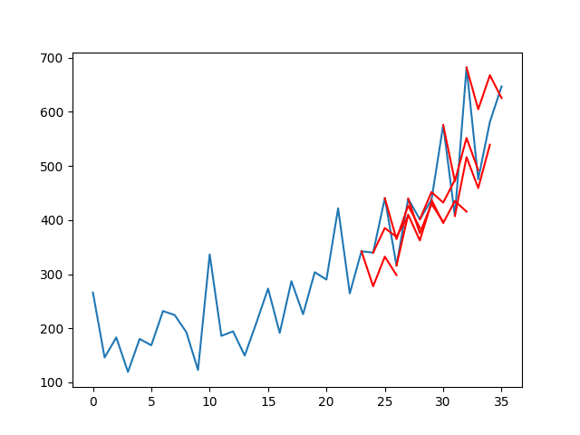
A line plot of the series (blue) with the forecasts (red) is also created.
The plot shows that although the skill of the model is better, some
of the forecasts are not very good and that there is plenty of room for
improvement.
Line Plot of Shampoo Sales Dataset with Multi-Step LSTM Forecasts
Extensions
There are some extensions you may consider if you are looking to push beyond this tutorial.
- Update LSTM. Change the example to refit or update
the LSTM as new data is made available. A 10s of training epochs should
be sufficient to retrain with a new observation.
- Tune the LSTM. Grid search some of the LSTM
parameters used in the tutorial, such as number of epochs, number of
neurons, and number of layers to see if you can further lift
performance.
- Seq2Seq. Use the encoder-decoder paradigm for LSTMs to forecast each sequence to see if this offers any benefit.
- Time Horizon. Experiment with forecasting different time horizons and see how the behavior of the network varies at different lead times.
Did you try any of these extensions?
Share your results in the comments; I’d love to hear about it.
Summary
In this tutorial, you discovered how to develop LSTM networks for multi-step time series forecasting.
Specifically, you learned:
- How to develop a persistence model for multi-step time series forecasting.
- How to develop an LSTM network for multi-step time series forecasting.
- How to evaluate and plot the results from multi-step time series forecasting.
Do you have any questions about multi-step time series forecasting with LSTMs?
Ask your questions in the comments below and I will do my best to answer.


No comments:
Post a Comment