A Tour of Recurrent Neural Network Algorithms for Deep Learning

 Recurrent neural networks, or RNNs, are a type of artificial neural network that add additional weights to the network to create cycles in the network graph in an effort to maintain an internal state.

The promise of adding state to neural networks is that they will be able to explicitly learn and exploit context in sequence prediction problems, such as problems with an order or temporal component.

In this post, you are going take a tour of recurrent neural networks used for deep learning.

After reading this post, you will know:

• How top recurrent neural networks used for deep learning work, such as LSTMs, GRUs, and NTMs.
• How top RNNs relate to the broader study of recurrence in artificial neural networks.
• How research in RNNs has led to state-of-the-art performance on a range of challenging problems.

  Overview

  We will start off by setting the scene for the field of recurrent neural networks.

  Next, we will take a closer look at LSTMs, GRUs, and NTM used for deep learning.

  We will then spend some time on advanced topics related to using RNNs for deep learning.

  • Recurrent Neural Networks
    • Fully Recurrent Networks
    • Recursive Neural Networks
    • Neural History Compressor
  • Long Short-Term Memory Networks
  • Gated Recurrent Unit Neural Networks
  • Neural Turing Machines

  Recurrent Neural Networks

  Let’s set the scene.

  Popular belief suggests that recurrence imparts a memory to the network topology.

  A better way to consider this is the training set contains examples with a set of inputs for the current training example. This is “conventional, e.g. a traditional multilayered Perceptron.

  X(i) -> y(i)

  But the training example is supplemented with a set of inputs from the previous example. This is “unconventional,” e.g. a recurrent neural network.

  [X(i-1), X(i)] -> y(i)

  As with all feed forward network paradigms, the issues are how to connect the input layer to the output layer, include feedback activations, and then train the construct to converge.

  Let’s now take a tour of the different types of recurrent neural networks, starting with very simple conceptions.

  Fully Recurrent Networks

  The layered topology of a multilayer Perceptron is preserved, but every element has a weighted connection to every other element in the architecture and has a single feedback connection to itself.

  Not all connections are trained and the extreme non-linearity of the error derivatives means conventional Backpropagation will not work, and so Backpropagation Through Time approaches or Stochastic Gradient Descent is employed.

  Also, see Bill Wilson’s Tensor Product Networks (1991).

  Recursive Neural Networks

  Recurrent neural networks are linear architectural variant of recursive networks.

  Recursion promotes branching in hierarchical feature spaces and the resulting network architecture mimics this as training proceeds.

  Training is achieved with Gradient Descent by sub-gradient methods.

  This is described in detail in R. Socher, et al., Parsing Natural Scenes and Natural Language with Recursive Neural Networks, 2011.

  Neural History Compressor

  Schmidhuber reported a very deep learner, first in 1991, that was able to perform credit assignment over hundreds of neural layers by unsupervised pre-training for a hierarchy of RNNs.

  Each RNN is trained unsupervised to predict the next input. Then only inputs generating an error are fed forward, conveying new information to the next RNN in the hierarchy, which then processes at a slower, self-organizing time scale.

  It was shown that no information is lost, just compressed. The RNN stack is a “deep generative model” of the data. The data can be reconstructed from the compressed form.

  See J. Schmidhuber, et al., Deep Learning in Neural Networks: An Overview, 2014.

  Backpropagation fails as the calculation of extremity of non-linear derivatives increases as the error is propagated backwards through large topologies, making credit assignment difficult, if not impossible.

  Need help with LSTMs for Sequence Prediction?

  Take my free 7-day email course and discover 6 different LSTM architectures (with code).

  Click to sign-up and also get a free PDF Ebook version of the course.

  Long Short-Term Memory Networks

  With conventional Back-Propagation Through Time (BPTT) or Real Time Recurrent Learning (RTTL), error signals flowing backward in time tend to either explode or vanish.

  The temporal evolution of the back-propagated error exponentially depends on the size of the weights. Weight explosion may lead to oscillating weights, while in vanishing causes learning to bridge long time lags and takes a prohibitive amount of time, or does not work at all.

  • LSTM is a novel recurrent network architecture training with an appropriate gradient-based learning algorithm.
  • LSTM is designed to overcome error back-flow problems. It can learn to bridge time intervals in excess of 1000 steps.
  • This true in presence of noisy, incompressible input sequences, without loss of short time lag capabilities.

  Error back-flow problems are overcome by an efficient, gradient-based algorithm for an architecture enforcing constant (thus neither exploding nor vanishing) error flow through internal states of special units. These units reduce the effects of the “Input Weight Conflict” and the “Output Weight Conflict.”

  The Input Weight Conflict: Provided the input is non-zero, the same incoming weight has to be used for both storing certain inputs and ignoring others, then will often receive conflicting weight update signals.

  These signals will attempt to make the weight participate in storing the input and protecting the input. This conflict makes learning difficult and calls for a more context-sensitive mechanism for controlling “write operations” through input weights.

  The Output Weight Conflict: As long as the output of a unit is non-zero, the weight on the output connection from this unit will attract conflicting weight update signals generated during sequence processing.

  These signals will attempt to make the outgoing weight participate in accessing the information stored in the processing unit and, at different times, protect the subsequent unit from being perturbed by the output of the unit being fed forward.

  These conflicts are not specific to long-term lags and can equally impinge on short-term lags. Of note though is that as lag increases, stored information must be protected from perturbation, especially in the advanced stages of learning.

  Network Architecture: Different types of units may convey useful information about the current state of the network. For instance, an input gate (output gate) may use inputs from other memory cells to decide whether to store (access) certain information in its memory cell.

  Memory cells contain gates. Gates are specific to the connection they mediate. Input gates work to remedy the Input Weight Conflict while Output Gates work to eliminate the Output Weight Conflict.

  Gates: Specifically, to alleviate the input and output weight conflicts and perturbations, a multiplicative input gate unit is introduced to protect the memory contents stored from perturbation by irrelevant inputs and a multiplicative output gate unit protects other units from perturbation by currently irrelevant memory contents stored.

  

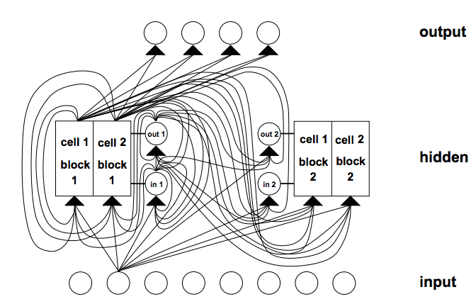
  Example of an LSTM net with 8 input units, 4 output units, and 2 memory cell blocks of size 2. in1 marks the input gate, out1 marks the output gate, and cell1 = block1 marks the first memory cell of block 1.
  Taken from Long Short-Term Memory, 1997.

  Connectivity in LSTM is complicated compared to the multilayer Perceptron because of the diversity of processing elements and the inclusion of feedback connections.

  Memory cell blocks: Memory cells sharing the same input gate and the same output gate form a structure called a “memory cell block”.

  Memory cell blocks facilitate information storage; as with conventional neural nets, it is not so easy to code a distributed input within a single cell. A memory cell block of size 1 is just a simple memory cell.

  Learning: A variant of Real Time Recurrent Learning (RTRL) that takes into account the altered, multiplicative dynamics caused by input and output gates is used to ensure non-decaying error back propagated through internal states of memory cells errors arriving at “memory cell net inputs” do not get propagated back further in time.

  Guessing: This stochastic approach can outperform many term lag algorithms. It has been established that many long-time lag tasks used in previous work can be solved more quickly by simple random weight guessing than by the proposed algorithms.

  See S. Hochreiter and J. Schmidhuber, Long-Short Term Memory, 1997.

  The most interesting application of LSTM Recurrent Neural Networks has been the work done with language processing. See the work of Gers for a comprehensive description.

  • F. Gers and J. Schmidhuber, LSTM Recurrent Networks Learn Simple Context Free and Context Sensitive Languages, 2001.
  • F. Gers, Long Short-Term Memory in Recurrent Neural Networks, Ph.D. Thesis, 2001.

  LSTM Limitations

  The efficient, truncated version of LSTM will not easily solve problems similar to “strongly delayed XOR.”

  Each memory cell block needs an input gate and an output gate. Not necessary in other recurrent approaches.

  Constant error flow through “Constant Error Carrousels” inside memory cells produces the same effect as a conventional feed-forward architecture being presented with the entire input string at once.

  LSTM is as flawed with the concept of “regency” as other feed-forward approaches. Additional counting mechanisms may be required if fine-precision counting time steps is needed.

  LSTM Advantages

  The algorithms ability to bridge long time lags is the result of constant error Backpropagation in the architecture’s memory cells.

  LSTM can approximate noisy problem domains, distributed representations, and continuous values.

  LSTM generalizes well over problem domains considered. This is important given some tasks are intractable for already established recurrent networks.

  Fine tuning of network parameters over the problem domains appears to be unnecessary.

  In terms of update complexity per weight and time steps, LSTM is essentially equivalent to BPTT.

  LSTMs are showing to be powerful, achieving state-of-the-art results in domains like machine translation.

  Gated Recurrent Unit Neural Networks

  Gated Recurrent Neural Networks have been successfully applied to sequential or temporal data.

  Most suitable for speech recognition, natural language processing, and machine translation, together with LSTM they have performed well with long sequence problem domains.

  Gating was considered in the LSTM topic and involves a gating network generating signals that act to control how the present input and previous memory work to update the current activation, and thereby the current network state.

  Gates are themselves weighted and are selectively updated according to an algorithm, throughout the learning phase.

  Gate networks introduce added computational expense in the form of increased complexity, and therefore added parameterization.

  The LSTM RNN architecture uses the computation of the simple RNN as an intermediate candidate for the internal memory cell (state). The Gated Recurrent Unit (GRU) RNN reduces the gating signals to two from the LSTM RNN model. The two gates are called an update gate and a reset gate.

  The gating mechanism in the GRU (and LSTM) RNN is a replica of the simple RNN in terms of parameterization. The weights corresponding to these gates are also updated using BPTT stochastic gradient descent as it seeks to minimize a cost function.

  Each parameter update will involve information pertaining to the state of the overall network. This can have detrimental effects.

  The concept of gating is explored further and extended with three new variant gating mechanisms.
  The three gating variants that have been considered are, GRU1 where each gate is computed using only the previous hidden state and the bias; GRU2, where each gate is computed using only the previous hidden state; and GRU3, where each gate is computed using only the bias. A significant reduction in parameters is observed with GRU3 yielding the smallest number.

  The three variants and the GRU RNN were benchmarked using data from the MNIST Database of handwritten digits and the IMDB movie review dataset.

  Two sequences lengths were generated from the MNIST dataset and one was generated from the IMDB dataset.

  The main driving signal of the gates appears to be the (recurrent) state as it contains essential information about other signals.

  The use of the stochastic gradient descent implicitly carries information about the network state. This may explain the relative success in using the bias alone in the gate signals as its adaptive update carries information about the state of the network.

  Gated variants explore the mechanisms of gating with limited evaluation of topologies.

  For more information see:

  • R. Dey and F. M. Salem, Gate-Variants of Gated Recurrent Unit (GRU) Neural Networks, 2017.
  • J. Chung, et al., Empirical Evaluation of Gated Recurrent Neural Networks on Sequence Modeling, 2014.

  Neural Turing Machines

  Neural Turing Machines extend the capabilities of neural networks by coupling them to external memory resources, which they can interact with through attention processes.

  The combined system is analogous to a Turing Machine or Von Neumann architecture, but is differentiable end-to-end, allowing it to be efficiently trained with gradient descent.

  Preliminary results demonstrate that Neural Turing Machines can infer simple algorithms, such as copying, sorting, and associative recall from input and output examples.

  RNNs stand out from other machine learning methods for their ability to learn and carry out complicated transformations of data over extended periods of time. Moreover, it is known that RNNs are Turing-Complete and therefore have the capacity to simulate arbitrary procedures, if properly wired.

  The capabilities of standard RNNs are extended to simplify the solution of algorithmic tasks. This enrichment is primarily via a large, addressable memory, so, by analogy to Turing’s enrichment of finite-state machines by an infinite memory tape, and so dubbed “Neural Turing Machine” (NTM).

  Unlike a Turing machine, an NTM is a differentiable computer that can be trained by gradient descent, yielding a practical mechanism for learning programs.

  

  NTM Architecture is generically shown above. During each update cycle, the controller network receives inputs from an external environment and emits outputs in response. It also reads to and writes from a memory matrix via a set of parallel read-and-write heads. The dashed line indicates the division between the NTM circuit and the outside world.
  Taken from Neural Turing Machines, 2014.

  Crucially, every component of the architecture is differentiable, making it straightforward to train with gradient descent. This was achieved this by defining ‘blurry’ read-and-write operations that interact to a greater or lesser degree with all the elements in memory (rather than addressing a single element, as in a normal Turing machine or digital computer).

  For more information see:

  • A. Graves, et al., Neural Turing Machines, 2014.
  • R. Greve, et al., Evolving Neural Turing Machines for Reward-based Learning, 2016.

  NTM Experiments

  The copy task tests whether NTM can store and recall a long sequence of arbitrary information. The network is presented with an input sequence of random binary vectors followed by a delimiter flag.

  The networks were trained to copy sequences of eight-bit random vectors where the sequence lengths were randomized between 1 and 20. The target sequence was simply a copy of the input sequence (without the delimiter flag).

  Repeat copy task extends copy by requiring the network to output the copied sequence a specified number of times and then emit an end-of-sequence marker. The main motivation was to see if the NTM could learn a simple nested function.

  The network receives random-length sequences of random binary vectors, followed by a scalar value indicating the desired number of copies, which appears on a separate input channel.

  Associative recall tasks involve organizing data arising from “indirection”, that is when one data item points to another. A list of items is constructed so that querying with one of the items demands that the network returns the subsequent item.

  A sequence of binary vectors that is bounded on the left and right by delimiter symbols is defined. After several items have been propagated to the network, the network is queried by showing a random item, and seeing if the network can produce the next item.

  Dynamic N-Grams task tests if the NTM can adapt quickly to new predictive distributions by using memory as a re-writable table that it could use to keep count of transition statistics, thereby emulating a conventional N-Gram model.

  Consider the set of all possible 6-Gram distributions over binary sequences. Each 6-Gram distribution can be expressed as a table of 32 numbers, specifying the probability that the next bit will be one, given all possible length five binary histories. A particular training sequence was generated by drawing 200 successive bits using the current lookup table. The network observes the sequence one bit at a time and is then asked to predict the next bit.

  Priority sort task tests the NTM’s ability to sort. A sequence of random binary vectors is input to the network along with a scalar priority rating for each vector. The priority is drawn uniformly from the range [-1, 1]. The target sequence contains the binary vectors sorted according to their priorities.

  NTMs have feed-forward architectures to LSTMs as one of their components.

  Summary

  In this post, you discovered recurrent neural networks for deep learning.

  Specifically, you learned:

  • How top recurrent neural networks used for deep learning work, such as LSTMs, GRUs, and NTMs.
  • How top RNNs relate to the broader study of recurrence in artificial neural networks.
  • How research in RNNs has lead to state-of-the-art performance on a range of challenging problems.

  This was a big post.

  Do you have any questions about RNNs for deep learning?
  Ask your questions in the comments below, and I will do my best to answer them.