Instability of Online Learning for Stateful LSTM for Time Series Forecasting

 Some neural network configurations can result in an unstable model.

This can make them hard to characterize and compare to other model configurations on the same problem using descriptive statistics.

One good example of a seemingly unstable model is the use of online learning (a batch size of 1) for a stateful Long Short-Term Memory (LSTM) model.

In this tutorial, you will discover how to explore the results of a stateful LSTM fit using online learning on a standard time series forecasting problem.

After completing this tutorial, you will know:

• How to design a robust test harness for evaluating LSTM models on time series forecasting problems.
• How to analyze a population of results, including summary statistics, spread, and distribution of results.
• How to analyze the impact of increasing the number of repeats for an experiment.

  Model Instability

  When you train the same network on the same data more than once, you may get very different results.

  This is because neural networks are initialized randomly and the optimization nature of how they are fit to the training data can result in different final weights within the network. These different networks can in turn result in varied predictions given the same input data.

  As a result, it is important to repeat any experiment on neural networks multiple times to find an averaged expected performance.

  For more on the stochastic nature of machine learning algorithms like neural networks, see the post:

  • Embrace Randomness in Machine Learning

  The batch size in a neural network defines how often the weights within the network are updated given exposure to a training dataset.

  A batch size of 1 means that the network weights are updated after each single row of training data. This is called online learning. The result is a network that can learn quickly, but a configuration that can be quite unstable.

  In this tutorial, we will explore the instability of online learning for a stateful LSTM configuration for time series forecasting.

  We will explore this by looking at the average performance of an LSTM configuration on a standard time series forecasting problem over a variable number of repeats of the experiment.

  That is, we will re-train the same model configuration on the same data many times and look at the performance of the model on a hold-out dataset and review how unstable the model can be.

  Tutorial Overview

  This tutorial is broken down into 6 parts. They are:

  1. Shampoo Sales Dataset
  2. Experimental Test Harness
  3. Code and Collect Results
  4. Basic Statistics on Results
  5. Repeats vs Test RMSE
  6. Review of Results

  Environment

  This tutorial assumes you have a Python SciPy environment installed. You can use either Python 2 or 3 with this example.

  This tutorial assumes you have Keras v2.0 or higher installed with either the TensorFlow or Theano backend.

  This tutorial also assumes you have scikit-learn, Pandas, NumPy, and Matplotlib installed.

  Next, let’s take a look at a standard time series forecasting problem that we can use as context for this experiment.

  Shampoo Sales Dataset

  This dataset describes the monthly number of sales of shampoo over a 3-year period.

  The units are a sales count and there are 36 observations. The original dataset is credited to Makridakis, Wheelwright, and Hyndman (1998).

  • Download the dataset.

  The example below loads and creates a plot of the loaded dataset.

  # load and plot dataset from pandas import read_csv from pandas import datetime from matplotlib import pyplot # load dataset def parser(x): return datetime.strptime('190'+x, '%Y-%m') series = read_csv('shampoo-sales.csv', header=0, parse_dates=[0], index_col=0, squeeze=True, date_parser=parser) # summarize first few rows print(series.head()) # line plot series.plot() pyplot.show()

  Running the example loads the dataset as a Pandas Series and prints the first 5 rows.

  Month 1901-01-01 266.0 1901-02-01 145.9 1901-03-01 183.1 1901-04-01 119.3 1901-05-01 180.3 Name: Sales, dtype: float64

  A line plot of the series is then created showing a clear increasing trend.

  

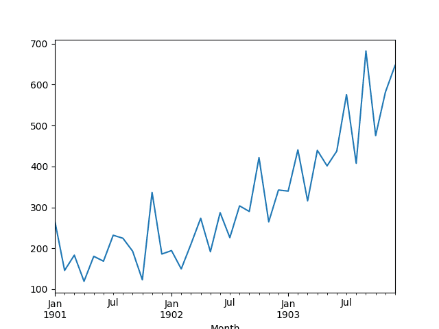
  Line Plot of Shampoo Sales Dataset

  Next, we will take a look at the LSTM configuration and test harness used in the experiment.

  Experimental Test Harness

  This section describes the test harness used in this tutorial.

  Data Split

  We will split the Shampoo Sales dataset into two parts: a training and a test set.

  The first two years of data will be taken for the training dataset and the remaining one year of data will be used for the test set.

  Models will be developed using the training dataset and will make predictions on the test dataset.

  The persistence forecast (naive forecast) on the test dataset achieves an error of 136.761 monthly shampoo sales. This provides a lower acceptable bound of performance on the test set.

  Model Evaluation

  A rolling-forecast scenario will be used, also called walk-forward model validation.

  Each time step of the test dataset will be walked one at a time. A model will be used to make a forecast for the time step, then the actual expected value from the test set will be taken and made available to the model for the forecast on the next time step.

  This mimics a real-world scenario where new Shampoo Sales observations would be available each month and used in the forecasting of the following month.

  This will be simulated by the structure of the train and test datasets.

  All forecasts on the test dataset will be collected and an error score calculated to summarize the skill of the model. The root mean squared error (RMSE) will be used as it punishes large errors and results in a score that is in the same units as the forecast data, namely monthly shampoo sales.

  Data Preparation

  Before we can fit an LSTM model to the dataset, we must transform the data.

  The following three data transforms are performed on the dataset prior to fitting a model and making a forecast.

  1. Transform the time series data so that it is stationary. Specifically a lag=1 differencing to remove the increasing trend in the data.
  2. Transform the time series into a supervised learning problem. Specifically the organization of data into input and output patterns where the observation at the previous time step is used as an input to forecast the observation at the current time step
  3. Transform the observations to have a specific scale. Specifically, to rescale the data to values between -1 and 1 to meet the default hyperbolic tangent activation function of the LSTM model.

  These transforms are inverted on forecasts to return them into their original scale before calculating and error score.

  LSTM Model

  We will use a base stateful LSTM model with 1 neuron fit for 1000 epochs.

  A batch size of 1 is required as we will be using walk-forward validation and making one-step forecasts for each of the final 12 months of test data.

  A batch size of 1 means that the model will be fit using online training (as opposed to batch training or mini-batch training). As a result, it is expected that the model fit will have some variance.

  Ideally, more training epochs would be used (such as 1500), but this was truncated to 1000 to keep run times reasonable.

  The model will be fit using the efficient ADAM optimization algorithm and the mean squared error loss function.

  Experimental Runs

  Each experimental scenario will be run 100 times and the RMSE score on the test set will be recorded from the end each run.

  All test RMSE scores are written to file for later analysis.

  Let’s dive into the experiments.

  Code and Collect Results

  The complete code listing is provided below.

  It may take a few hours to run on modern hardware.

  from pandas import DataFrame from pandas import Series from pandas import concat from pandas import read_csv from pandas import datetime from sklearn.metrics import mean_squared_error from sklearn.preprocessing import MinMaxScaler from keras.models import Sequential from keras.layers import Dense from keras.layers import LSTM from math import sqrt import matplotlib import numpy from numpy import concatenate   # date-time parsing function for loading the dataset def parser(x): return datetime.strptime('190'+x, '%Y-%m')   # frame a sequence as a supervised learning problem def timeseries_to_supervised(data, lag=1): df = DataFrame(data) columns = [df.shift(i) for i in range(1, lag+1)] columns.append(df) df = concat(columns, axis=1) return df   # create a differenced series def difference(dataset, interval=1): diff = list() for i in range(interval, len(dataset)): value = dataset[i] - dataset[i - interval] diff.append(value) return Series(diff)   # invert differenced value def inverse_difference(history, yhat, interval=1): return yhat + history[-interval]   # scale train and test data to [-1, 1] def scale(train, test): # fit scaler scaler = MinMaxScaler(feature_range=(-1, 1)) scaler = scaler.fit(train) # transform train train = train.reshape(train.shape[0], train.shape[1]) train_scaled = scaler.transform(train) # transform test test = test.reshape(test.shape[0], test.shape[1]) test_scaled = scaler.transform(test) return scaler, train_scaled, test_scaled   # inverse scaling for a forecasted value def invert_scale(scaler, X, yhat): new_row = [x for x in X] + [yhat] array = numpy.array(new_row) array = array.reshape(1, len(array)) inverted = scaler.inverse_transform(array) return inverted[0, -1]   # fit an LSTM network to training data def fit_lstm(train, batch_size, nb_epoch, neurons): X, y = train[:, 0:-1], train[:, -1] X = X.reshape(X.shape[0], 1, X.shape[1]) model = Sequential() model.add(LSTM(neurons, batch_input_shape=(batch_size, X.shape[1], X.shape[2]), stateful=True)) model.add(Dense(1)) model.compile(loss='mean_squared_error', optimizer='adam') for i in range(nb_epoch): model.fit(X, y, epochs=1, batch_size=batch_size, verbose=0, shuffle=False) model.reset_states() return model   # make a one-step forecast def forecast_lstm(model, batch_size, X): X = X.reshape(1, 1, len(X)) yhat = model.predict(X, batch_size=batch_size) return yhat[0,0]   # run a repeated experiment def experiment(repeats, series): # transform data to be stationary raw_values = series.values diff_values = difference(raw_values, 1) # transform data to be supervised learning supervised = timeseries_to_supervised(diff_values, 1) supervised_values = supervised.values[1:,:] # split data into train and test-sets train, test = supervised_values[0:-12, :], supervised_values[-12:, :] # transform the scale of the data scaler, train_scaled, test_scaled = scale(train, test) # run experiment error_scores = list() for r in range(repeats): # fit the base model lstm_model = fit_lstm(train_scaled, 1, 1000, 1) # forecast test dataset predictions = list() for i in range(len(test_scaled)): # predict X, y = test_scaled[i, 0:-1], test_scaled[i, -1] yhat = forecast_lstm(lstm_model, 1, X) # invert scaling yhat = invert_scale(scaler, X, yhat) # invert differencing yhat = inverse_difference(raw_values, yhat, len(test_scaled)+1-i) # store forecast predictions.append(yhat) # report performance rmse = sqrt(mean_squared_error(raw_values[-12:], predictions)) print('%d) Test RMSE: %.3f' % (r+1, rmse)) error_scores.append(rmse) return error_scores   # execute the experiment def run(): # load dataset series = read_csv('shampoo-sales.csv', header=0, parse_dates=[0], index_col=0, squeeze=True, date_parser=parser) # experiment repeats = 100 results = DataFrame() # run experiment results['results'] = experiment(repeats, series) # summarize results print(results.describe()) # save results results.to_csv('experiment_stateful.csv', index=False)   # entry point run()

  Running the experiment saves the RMSE scores of the fit model on the test dataset.

  Results are saved to the file “experiment_stateful.csv“.

  Note: Your results may vary given the stochastic nature of the algorithm or evaluation procedure, or differences in numerical precision. Consider running the example a few times and compare the average outcome.

  A truncated listing of the results is provided below.

  ... 116.39769471284067 105.0459745537738 93.57827109861229 128.973001927212 97.02915084460737 198.56877142225886 113.09568645243242 97.84127724751188 124.60413895331735 111.62139008607713

  Basic Statistics on Results

  We can start off by calculating some basic statistics on the entire population of 100 test RMSE scores.

  Generally, we expect machine learning results to have a Gaussian distribution. This allows us to report the mean and standard deviation of a model and indicate a confidence interval for the model when making predictions on unseen data.

  The snippet below loads the result file and calculates some descriptive statistics.

  from pandas import DataFrame from pandas import read_csv from numpy import mean from numpy import std from matplotlib import pyplot # load results file results = read_csv('experiment_stateful.csv', header=0) # descriptive stats print(results.describe()) # box and whisker plot results.boxplot() pyplot.show()

  Running the example prints descriptive statistics from the results.

  Note: Your results may vary given the stochastic nature of the algorithm or evaluation procedure, or differences in numerical precision. Consider running the example a few times and compare the average outcome.

  We can see that on average, the configuration achieved an RMSE of about 107 monthly shampoo sales with a standard deviation of about 17.

  We can also see that the best test RMSE observed was about 90 sales, whereas the worse was just under 200, which is quite a spread of scores.

  results count  100.000000 mean   107.051146 std     17.694512 min     90.407323 25%     96.630800 50%    102.603908 75%    111.199574 max    198.568771

  To get a better idea of the spread of the data, a box and whisker plot is also created.

  The plot shows the median (green line), middle 50% of the data (box), and outliers (dots). We can see quite a spread to the data towards poor RMSE scores.

  

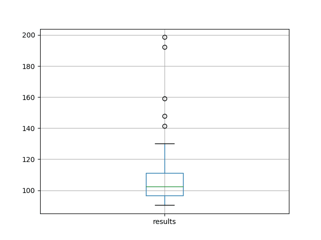
  Box and Whisker Plot of 100 Test RMSE Scores on the Shampoo Sales Dataset

  A histogram of the raw result values is also created.

  The plot suggests a skewed or even an exponential distribution with a mass around an RMSE of 100 and a long tail leading out towards an RMSE of 200.

  The distribution of the results are clearly not Gaussian. This is unfortunate, as the mean and standard deviation cannot be used directly to estimate a confidence interval for the model (e.g. 95% confidence as 2x the standard deviation around the mean).

  The skewed distribution also highlights that the median (50th percentile) would be a better central tendency to use instead of the mean for these results. The median should be more robust to outlier results than the mean.

  

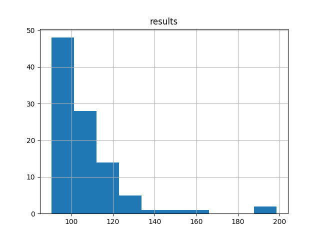
  Histogram of Test RMSE Scores on Shampoo Sales Dataset

  Repeats vs Test RMSE

  We can start to look at how the summary statistics for the experiment change as the number of repeats is increased from 1 to 100.

  We can accumulate the test RMSE scores and calculate descriptive statistics. For example, the score from one repeat, the scores from the first and second repeats, the scores from the first 3 repeats, and so on to 100 repeats.

  We can review how the central tendency changes as the number of repeats is increased as a line plot. We’ll look at both the mean and median.

  Generally, we would expect that as the number of repeats of the experiment is increased, the distribution would increasingly better match the underlying distribution, including the central tendency, such as the mean.

  The complete code listing is provided below.

  from pandas import DataFrame from pandas import read_csv from numpy import median from numpy import mean from matplotlib import pyplot import numpy # load results file results = read_csv('experiment_stateful.csv', header=0) values = results.values # collect cumulative stats medians, means = list(), list() for i in range(1,len(values)+1): data = values[0:i, 0] mean_rmse, median_rmse = mean(data), median(data) means.append(mean_rmse) medians.append(median_rmse) print(i, mean_rmse, median_rmse) # line plot of cumulative values line1, = pyplot.plot(medians, label='Median RMSE') line2, = pyplot.plot(means, label='Mean RMSE') pyplot.legend(handles=[line1, line2]) pyplot.show()

  The cumulative size of the distribution, mean, and median is printed as the number of repeats is increased.

  Note: Your results may vary given the stochastic nature of the algorithm or evaluation procedure, or differences in numerical precision. Consider running the example a few times and compare the average outcome.

  A truncated output is listed below.

  ... 90 105.759546832 101.477640071 91 105.876449555 102.384620485 92 105.867422653 102.458057114 93 105.735281239 102.384620485 94 105.982491033 102.458057114 95 105.888245347 102.384620485 96 106.853667494 102.458057114 97 106.918018205 102.531493742 98 106.825398399 102.458057114 99 107.004981637 102.531493742 100 107.051145721 102.603907965

  A line plot is also created showing how the mean and median change as the number of repeats is increased.

  The results show that the mean is more influenced by outlier results than the median, as expected.

  We can see that the median appears quite stable down around 99-100. This jumps to 102 towards the end of the plot suggesting a string of worse RMSE scores at later repeats.

  

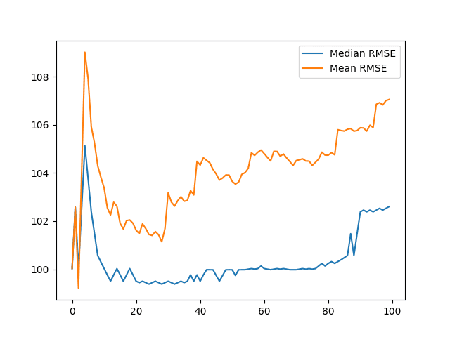
  Line Plots of Mean and Median Test RMSE vs Number of Repeats

  Review of Results

  We made some useful observations from 100 repeats of a stateful LSTM on a standard time series forecasting problem.

  Specifically:

  • We observed that the distribution of results is not Gaussian. It may be a skewed Gaussian or an exponential distribution with a long tail and outliers.
  • We observed that the distribution of results did not stabilize with the increase of repeats from 1 to 100.

  The observations suggest a few important properties:

  • The choice of online learning for the LSTM and problem results in a relatively unstable model.
  • The chosen number of repeats (100) may not be sufficient to characterize the behavior of the model.

  This is a useful finding as it would be a mistake to make strong conclusions about the model from 100 or fewer repeats of the experiment.

  This is an important caution to consider when describing your own machine learning results.

  This suggests some extensions to this experiment, such as:

  • Explore the impact of the number of repeats on a more stable model, such as one using batch or mini-batch learning.
  • Increase the number of repeats to thousands or more in an attempt to account for the general instability of the model with online learning.

  Summary

  In this tutorial, you discovered how to analyze experimental results from LSTM models fit using online learning.

  You learned:

  • How to design a robust test harness for evaluating LSTM models on time series forecast problems.
  • How to analyze experimental results, including summary statistics.
  • How to analyze the impact of increasing the number of experiment repeats and how to identify an unstable model.

  Do you have any questions?
  Ask your questions in the comments below and I will do my best to answer.