How to Update LSTM Networks During Training for Time Series Forecasting

 A benefit of using neural network models for time series forecasting is that the weights can be updated as new data becomes available.

In this tutorial, you will discover how you can update a Long Short-Term Memory (LSTM) recurrent neural network with new data for time series forecasting.

After completing this tutorial, you will know:

• How to update an LSTM neural network with new data.
• How to develop a test harness to evaluate different update schemes.
• How to interpret the results from updating LSTM networks with new data.

  Tutorial Overview

  This tutorial is divided into 9 parts. They are:

  1. Shampoo Sales Dataset
  2. Experimental Test Harness
  3. Experiment: No Updates
  4. Experiment: 2 Update Epochs
  5. Experiment: 5 Update Epochs
  6. Experiment: 10 Update Epochs
  7. Experiment: 20 Update Epochs
  8. Experiment: 50 Update Epochs
  9. Comparison of Results

  Environment

  This tutorial assumes you have a Python SciPy environment installed. You can use either Python 2 or 3 with this example.

  This tutorial assumes you have Keras v2.0 or higher installed with either the TensorFlow or Theano backend.

  This tutorial also assumes you have scikit-learn, Pandas, NumPy, and Matplotlib installed.

  If you need help setting up your Python environment, see this post:

  • How to Setup a Python Environment for Machine Learning and Deep Learning with Anaconda

  Shampoo Sales Dataset

  This dataset describes the monthly number of sales of shampoo over a 3-year period.

  The units are a sales count and there are 36 observations. The original dataset is credited to Makridakis, Wheelwright, and Hyndman (1998).

  • Download the dataset.

  The example below loads and creates a plot of the loaded dataset.

  # load and plot dataset from pandas import read_csv from pandas import datetime from matplotlib import pyplot # load dataset def parser(x): return datetime.strptime('190'+x, '%Y-%m') series = read_csv('shampoo-sales.csv', header=0, parse_dates=[0], index_col=0, squeeze=True, date_parser=parser) # summarize first few rows print(series.head()) # line plot series.plot() pyplot.show()

  Running the example loads the dataset as a Pandas Series and prints the first 5 rows.

  Month 1901-01-01 266.0 1901-02-01 145.9 1901-03-01 183.1 1901-04-01 119.3 1901-05-01 180.3 Name: Sales, dtype: float64

  A line plot of the series is then created showing a clear increasing trend.

  

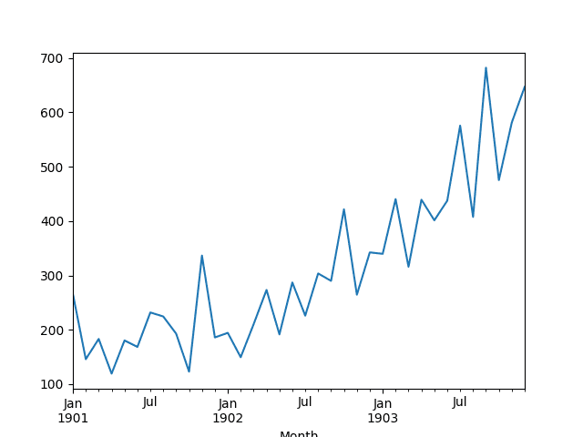
  Line Plot of Shampoo Sales Dataset

  Next, we will take a look at the LSTM configuration and test harness used in the experiment.

  Need help with Deep Learning for Time Series?

  Take my free 7-day email crash course now (with sample code).

  Click to sign-up and also get a free PDF Ebook version of the course.

  Experimental Test Harness

  This section describes the test harness used in this tutorial.

  Data Split

  We will split the Shampoo Sales dataset into two parts: a training and a test set.

  The first two years of data will be taken for the training dataset and the remaining one year of data will be used for the test set.

  Models will be developed using the training dataset and will make predictions on the test dataset.

  The persistence forecast (naive forecast) on the test dataset achieves an error of 136.761 monthly shampoo sales. This provides an acceptable lower bound of performance on the test set.

  Model Evaluation

  A rolling-forecast scenario will be used, also called walk-forward model validation.

  Each time step of the test dataset will be walked one at a time. A model will be used to make a forecast for the time step, then the actual expected value from the test set will be taken and made available to the model for the forecast on the next time step.

  This mimics a real-world scenario where new Shampoo Sales observations would be available each month and used in the forecasting of the following month.

  This will be simulated by the structure of the train and test datasets.

  All forecasts on the test dataset will be collected and an error score calculated to summarize the skill of the model. The root mean squared error (RMSE) will be used as it punishes large errors and results in a score that is in the same units as the forecast data, namely monthly shampoo sales.

  Data Preparation

  Before we can fit an LSTM model to the dataset, we must transform the data.

  The following three data transforms are performed on the dataset prior to fitting a model and making a forecast.

  1. Transform the time series data so that it is stationary. Specifically, a lag=1 differencing to remove the increasing trend in the data.
  2. Transform the time series into a supervised learning problem. Specifically, the organization of data into input and output patterns where the observation at the previous time step is used as an input to forecast the observation at the current time step
  3. Transform the observations to have a specific scale. Specifically, to rescale the data to values between -1 and 1 to meet the default hyperbolic tangent activation function of the LSTM model.

  These transforms are inverted on forecasts to return them into their original scale before calculating an error score.

  LSTM Model

  We will use an LSTM model with 1 neuron fit for 500 epochs.

  A batch size of 1 is required as we will be using walk-forward validation and making one-step forecasts for each of the final 12 months of data.

  A batch size of 1 means that the model will be fit using online training (as opposed to batch training or mini-batch training). As a result, it is expected that the model fit will have some variance.

  Ideally, more training epochs would be used (such as 1000 or 1500), but this was truncated to 500 to keep run times reasonable.

  The model will be fit using the efficient ADAM optimization algorithm and the mean squared error loss function.

  Experimental Runs

  Each experimental scenario will be run 10 times.

  The reason for this is that the random initial conditions for an LSTM network can result in very different performance each time a given configuration is trained.

  Let’s dive into the experiments.

  Experiment: No Updates

  In this first experiment, we will evaluate an LSTM trained once and reused to make a forecast for each time step.

  We will call this the ‘no updates model‘ or the ‘fixed model‘ as no updates will be made once the model is first fit on the training data. This provides a baseline of performance that we would expect experiments that make modest updates to the model to outperform.

  The complete code listing is provided below.

  from pandas import DataFrame from pandas import Series from pandas import concat from pandas import read_csv from pandas import datetime from sklearn.metrics import mean_squared_error from sklearn.preprocessing import MinMaxScaler from keras.models import Sequential from keras.layers import Dense from keras.layers import LSTM from math import sqrt import matplotlib import numpy from numpy import concatenate   # date-time parsing function for loading the dataset def parser(x): return datetime.strptime('190'+x, '%Y-%m')   # frame a sequence as a supervised learning problem def timeseries_to_supervised(data, lag=1): df = DataFrame(data) columns = [df.shift(i) for i in range(1, lag+1)] columns.append(df) df = concat(columns, axis=1) df = df.drop(0) return df   # create a differenced series def difference(dataset, interval=1): diff = list() for i in range(interval, len(dataset)): value = dataset[i] - dataset[i - interval] diff.append(value) return Series(diff)   # invert differenced value def inverse_difference(history, yhat, interval=1): return yhat + history[-interval]   # scale train and test data to [-1, 1] def scale(train, test): # fit scaler scaler = MinMaxScaler(feature_range=(-1, 1)) scaler = scaler.fit(train) # transform train train = train.reshape(train.shape[0], train.shape[1]) train_scaled = scaler.transform(train) # transform test test = test.reshape(test.shape[0], test.shape[1]) test_scaled = scaler.transform(test) return scaler, train_scaled, test_scaled   # inverse scaling for a forecasted value def invert_scale(scaler, X, yhat): new_row = [x for x in X] + [yhat] array = numpy.array(new_row) array = array.reshape(1, len(array)) inverted = scaler.inverse_transform(array) return inverted[0, -1]   # fit an LSTM network to training data def fit_lstm(train, batch_size, nb_epoch, neurons): X, y = train[:, 0:-1], train[:, -1] X = X.reshape(X.shape[0], 1, X.shape[1]) model = Sequential() model.add(LSTM(neurons, batch_input_shape=(batch_size, X.shape[1], X.shape[2]), stateful=True)) model.add(Dense(1)) model.compile(loss='mean_squared_error', optimizer='adam') for i in range(nb_epoch): model.fit(X, y, epochs=1, batch_size=batch_size, verbose=0, shuffle=False) model.reset_states() return model   # make a one-step forecast def forecast_lstm(model, batch_size, X): X = X.reshape(1, 1, len(X)) yhat = model.predict(X, batch_size=batch_size) return yhat[0,0]   # run a repeated experiment def experiment(repeats, series): # transform data to be stationary raw_values = series.values diff_values = difference(raw_values, 1) # transform data to be supervised learning supervised = timeseries_to_supervised(diff_values, 1) supervised_values = supervised.values # split data into train and test-sets train, test = supervised_values[0:-12], supervised_values[-12:] # transform the scale of the data scaler, train_scaled, test_scaled = scale(train, test) # run experiment error_scores = list() for r in range(repeats): # fit the base model lstm_model = fit_lstm(train_scaled, 1, 500, 1) # forecast test dataset predictions = list() for i in range(len(test_scaled)): # predict X, y = test_scaled[i, 0:-1], test_scaled[i, -1] yhat = forecast_lstm(lstm_model, 1, X) # invert scaling yhat = invert_scale(scaler, X, yhat) # invert differencing yhat = inverse_difference(raw_values, yhat, len(test_scaled)+1-i) # store forecast predictions.append(yhat) # report performance rmse = sqrt(mean_squared_error(raw_values[-12:], predictions)) print('%d) Test RMSE: %.3f' % (r+1, rmse)) error_scores.append(rmse) return error_scores   # execute the experiment def run(): # load dataset series = read_csv('shampoo-sales.csv', header=0, parse_dates=[0], index_col=0, squeeze=True, date_parser=parser) # experiment repeats = 10 results = DataFrame() # run experiment results['results'] = experiment(repeats, series) # summarize results print(results.describe()) # save results results.to_csv('experiment_fixed.csv', index=False)   # entry point run()

  Running the example stores the RMSE scores calculated on the test dataset using walk-forward validation. These are stored in a file called experiment_fixed.csv for later analysis. A summary of the scores is printed, shown below.

  Note: Your results may vary given the stochastic nature of the algorithm or evaluation procedure, or differences in numerical precision. Consider running the example a few times and compare the average outcome.

  The results suggest an average performance that outperforms the persistence model showing a test RMSE of 109.565465 compared to 136.761 monthly shampoo sales for persistence.

  results count   10.000000 mean   109.565465 std     14.329646 min     95.357198 25%     99.870983 50%    104.864387 75%    113.553952 max    138.261929

  Next, we will start looking at configurations that make updates to the model during the walk-forward validation.

  Experiment: 2 Update Epochs

  In this experiment, we fit the model on all of the training data, then update the model after each forecast during the walk-forward validation.

  Each test pattern used to elicit a forecast in the test dataset is then added to the training dataset and the model is updated.

  In this case, the model is fit for an additional 2 training epochs before making the next forecast.

  The same code listing as was used in the first experiment is used. The changes to the code listing are shown below.

  # Update LSTM model def update_model(model, train, batch_size, updates): X, y = train[:, 0:-1], train[:, -1] X = X.reshape(X.shape[0], 1, X.shape[1]) for i in range(updates): model.fit(X, y, epochs=1, batch_size=batch_size, verbose=0, shuffle=False) model.reset_states()   # run a repeated experiment def experiment(repeats, series, updates): # transform data to be stationary raw_values = series.values diff_values = difference(raw_values, 1) # transform data to be supervised learning supervised = timeseries_to_supervised(diff_values, 1) supervised_values = supervised.values # split data into train and test-sets train, test = supervised_values[0:-12], supervised_values[-12:] # transform the scale of the data scaler, train_scaled, test_scaled = scale(train, test) # run experiment error_scores = list() for r in range(repeats): # fit the base model lstm_model = fit_lstm(train_scaled, 1, 500, 1) # forecast test dataset train_copy = numpy.copy(train_scaled) predictions = list() for i in range(len(test_scaled)): # update model if i > 0: update_model(lstm_model, train_copy, 1, updates) # predict X, y = test_scaled[i, 0:-1], test_scaled[i, -1] yhat = forecast_lstm(lstm_model, 1, X) # invert scaling yhat = invert_scale(scaler, X, yhat) # invert differencing yhat = inverse_difference(raw_values, yhat, len(test_scaled)+1-i) # store forecast predictions.append(yhat) # add to training set train_copy = concatenate((train_copy, test_scaled[i,:].reshape(1, -1))) # report performance rmse = sqrt(mean_squared_error(raw_values[-12:], predictions)) print('%d) Test RMSE: %.3f' % (r+1, rmse)) error_scores.append(rmse) return error_scores   # execute the experiment def run(): # load dataset series = read_csv('shampoo-sales.csv', header=0, parse_dates=[0], index_col=0, squeeze=True, date_parser=parser) # experiment repeats = 10 results = DataFrame() # run experiment updates = 2 results['results'] = experiment(repeats, series, updates) # summarize results print(results.describe()) # save results results.to_csv('experiment_update_2.csv', index=False)   # entry point run()

  Note: Your results may vary given the stochastic nature of the algorithm or evaluation procedure, or differences in numerical precision. Consider running the example a few times and compare the average outcome.

  Running the experiment saves the final test RMSE scores in “experiment_update_2.csv” and prints summary statistics of the results, listed below.

  results count   10.000000 mean    99.566270 std     10.511337 min     87.771671 25%     93.925243 50%     97.903038 75%    101.213058 max    124.748746

  Experiment: 5 Update Epochs

  This experiments repeats the above update experiment and trains the model for an additional 5 epochs after each test pattern is added to the training dataset.

  Note: Your results may vary given the stochastic nature of the algorithm or evaluation procedure, or differences in numerical precision. Consider running the example a few times and compare the average outcome.

  Running the experiment saves the final test RMSE scores in “experiment_update_5.csv” and prints summary statistics of the results, listed below.

  results count   10.000000 mean   101.094469 std      9.422711 min     91.642706 25%     94.593701 50%     98.954743 75%    104.998420 max    123.651985

  Experiment: 10 Update Epochs

  This experiments repeats the above update experiment and trains the model for an additional 10 epochs after each test pattern is added to the training dataset.

  Note: Your results may vary given the stochastic nature of the algorithm or evaluation procedure, or differences in numerical precision. Consider running the example a few times and compare the average outcome.

  Running the experiment saves the final test RMSE scores in “experiment_update_10.csv” and prints summary statistics of the results, listed below.

  results count   10.000000 mean   108.806418 std     21.707665 min     92.161703 25%     94.872009 50%     99.652295 75%    112.607260 max    159.921749

  Experiment: 20 Update Epochs

  This experiments repeats the above update experiment and trains the model for an additional 20 epochs after each test pattern is added to the training dataset.

  Note: Your results may vary given the stochastic nature of the algorithm or evaluation procedure, or differences in numerical precision. Consider running the example a few times and compare the average outcome.

  Running the experiment saves the final test RMSE scores in “experiment_update_20.csv” and prints summary statistics of the results, listed below.

  results count   10.000000 mean   112.070895 std     16.631902 min     96.822760 25%    101.790705 50%    103.380896 75%    119.479211 max    140.828410

  Experiment: 50 Update Epochs

  This experiments repeats the above update experiment and trains the model for an additional 50 epochs after each test pattern is added to the training dataset.

  Note: Your results may vary given the stochastic nature of the algorithm or evaluation procedure, or differences in numerical precision. Consider running the example a few times and compare the average outcome.

  Running the experiment saves the final test RMSE scores in “experiment_update_50.csv” and prints summary statistics of the results, listed below.

  results count   10.000000 mean   110.721971 std     22.788192 min     93.362982 25%     96.833140 50%     98.411940 75%    123.793652 max    161.463289

  Comparison of Results

  In this section, we compare the results saved from the previous experiments.

  We load each of the saved results, summarize the results with descriptive statistics, and compare the results using box and whisker plots.

  The complete code listing is provided below.

  from pandas import DataFrame from pandas import read_csv from matplotlib import pyplot # load results into a dataframe filenames = ['experiment_fixed.csv', 'experiment_update_2.csv', 'experiment_update_5.csv', 'experiment_update_10.csv', 'experiment_update_20.csv', 'experiment_update_50.csv'] results = DataFrame() for name in filenames: results[name[11:-4]] = read_csv(name, header=0) # describe all results print(results.describe()) # box and whisker plot results.boxplot() pyplot.show()

  Running the example first calculates and prints descriptive statistics for each of the experimental results.

  Note: Your results may vary given the stochastic nature of the algorithm or evaluation procedure, or differences in numerical precision. Consider running the example a few times and compare the average outcome.

  If we look at the average performance, we can see that the fixed model provides a good baseline of performance, but we see that a modest number of update epochs (20 and 50) produce worse test set RMSE on average.

  We see that a small number of update epochs result in better overall test set performance, specifically 2 epochs followed by 5 epochs. This is encouraging.

  fixed    update_2    update_5   update_10   update_20   update_50 count   10.000000   10.000000   10.000000   10.000000   10.000000   10.000000 mean   109.565465   99.566270  101.094469  108.806418  112.070895  110.721971 std     14.329646   10.511337    9.422711   21.707665   16.631902   22.788192 min     95.357198   87.771671   91.642706   92.161703   96.822760   93.362982 25%     99.870983   93.925243   94.593701   94.872009  101.790705   96.833140 50%    104.864387   97.903038   98.954743   99.652295  103.380896   98.411940 75%    113.553952  101.213058  104.998420  112.607260  119.479211  123.793652 max    138.261929  124.748746  123.651985  159.921749  140.828410  161.463289

  A box and whisker plot is also created that compares the distribution of test RMSE results from each experiment.

  The plot highlights the median (green line) as well as the middle 50% of the data (box) for each experiment. The plot tells the same story as the average performance, suggesting that a small number of training epochs (2 or 5 epochs) result in the best overall test RMSE.

  The plot shows a rise in test RMSE as the number of updates increases to 20 epochs, then back down again for 50 epochs. This might be a sign of significant further training improving the model (11 * 50 epochs) or an artifact of the small number of repeats (10).

  

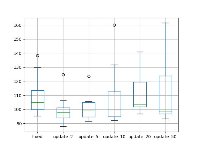
  Box and Whisker Plots Comparing the Number of Update Epochs

  It is important to point out that these results are specific to the model configuration and this dataset.

  It is hard to generalize these results beyond this specific example, although these experiments do provide a framework for performing similar experiments on your own predictive modeling problem.

  Extensions

  This section lists ideas for extensions to the experiments in this section.

  • Statistical Significance Tests. We could calculate pairwise statistical significance tests, such as the Student t-test, to see if the differences between the means in the populations of results are statistically significant or not.
  • More Repeats. We could increase the number of repeats from 10 to 30, 100, or more in an attempt to make the findings more robust.
  • More Epochs. The base LSTM model was only fit for 500 epochs with online training and it is believed that additional training epochs will result in a more accurate baseline model. The number of epochs was cut to decrease experiment run time.
  • Compare to more Epochs. The results for experiments that update the model should be compared directly to experiments of a fixed model that uses the same number of overall epochs to see if adding the additional test patterns to the training dataset makes any noticeable difference. For example, 2 update epochs for each test pattern could be compared to a fixed model trained for 500 + (12-1) * 2) or 522 epochs, an update model 5 compared to a fixed model fit for 500 + (12-1) * 5) or 555 epochs, and so on.
  • Completely New Model. Add an experiment where a new model is fit after each test pattern is added to the training dataset. This was attempted, but the extended run time prevented the results being collected prior to finalizing this tutorial. This would be expected to provide an interesting point of comparison to the update and fixed models.

  Did you explore any of these extensions?
  Report your results in the comments; I’d love to hear what you discovered.

  Summary

  In this tutorial, you discovered how to update an LSTM network as new data becomes available for time series forecasting in Python.

  Specifically, you learned:

  • How to design a systematic set of experiments to explore the effect of updating LSTM models.
  • How to update an LSTM model as new data becomes available.
  • That updates to an LSTM model can result in a more effective predictive model, but careful calibration is required on your forecast problem.

  Do you have any questions?
  Ask your questions in the comments below and I will do my best to answer.