How to Seed State for LSTMs for Time Series Forecasting in Python

 Long Short-Term Memory networks, or LSTMs, are a powerful type of recurrent neural network capable of learning long sequences of observations.

A promise of LSTMs is that they may be effective at time series forecasting, although the method is known to be difficult to configure and use for these purposes.

A key feature of LSTMs is that they maintain an internal state that can aid in the forecasting. This raises the question of how best to seed the state of a fit LSTM model prior to making a forecast.

In this tutorial, you will discover how to design, execute, and interpret the results from an experiment to explore whether it is better to seed the state of a fit LSTM from the training dataset or to use no prior state.

After completing this tutorial, you will know:

• About the open question of how to best initialize the state of a fit LSTM for forecasting.
• How to develop a robust test harness for evaluating LSTM models on univariate time series forecasting problems.
• How to determine whether or not seeding the state of your LSTM prior to forecasting is a good idea on your time series forecasting problem.

  Tutorial Overview

  This tutorial is broken down into 5 parts; they are:

  1. Seeding LSTM State
  2. Shampoo Sales Dataset
  3. LSTM Model and Test Harness
  4. Code Listing
  5. Experimental Results

  Environment

  This tutorial assumes you have a Python SciPy environment installed. You can use either Python 2 or 3 with this example.

  You must have Keras (version 2.0 or higher) installed with either the TensorFlow or Theano backend.

  The tutorial also assumes you have scikit-learn, Pandas, NumPy, and Matplotlib installed.

  If you need help setting up your Python environment, see this post:

  • How to Setup a Python Environment for Machine Learning and Deep Learning with Anaconda

  Seeding LSTM State

  When using stateless LSTMs in Keras, you have fine-grained control over when the internal state of the model is cleared.

  This is achieved using the model.reset_states() function.

  When training a stateful LSTM, it is important to clear the state of the model between training epochs. This is so that the state built up during training over the epoch is commensurate with the sequence of observations in the epoch.

  Given that we have this fine-grained control, there is a question as to whether or not and how to initialize the state of the LSTM prior to making a forecast.

  The options are:

  • Reset state prior to forecasting.
  • Initialize state with the training datasets prior to forecasting.

  It is assumed that initializing the state of the model using the training data would be superior, but this needs to be confirmed with experimentation.

  Additionally, there may be multiple ways to seed this state; for example:

  • Complete a training epoch, including weight updates. For example, do not reset at the end of the last training epoch.
  • Complete a forecast of the training data.

  Generally, it is believed that both of these approaches would be somewhat equivalent. The latter of forecasting the training dataset is preferred because it does not require any modification to network weights and could be a repeatable procedure for an immutable network saved to file.

  In this tutorial, we will consider the difference between:

  • Forecasting a test dataset using a fit LSTM with no state (e.g. after a reset).
  • Forecasting a test dataset with a fit LSTM with state after having forecast the training dataset.

  Next, let’s take a look at a standard time series dataset we will use in this experiment.

  Shampoo Sales Dataset

  This dataset describes the monthly number of sales of shampoo over a 3-year period.

  The units are a sales count and there are 36 observations. The original dataset is credited to Makridakis, Wheelwright, and Hyndman (1998).

  • Download the dataset.

  The example below loads and creates a plot of the loaded dataset.

  # load and plot dataset from pandas import read_csv from pandas import datetime from matplotlib import pyplot # load dataset def parser(x): return datetime.strptime('190'+x, '%Y-%m') series = read_csv('shampoo-sales.csv', header=0, parse_dates=[0], index_col=0, squeeze=True, date_parser=parser) # summarize first few rows print(series.head()) # line plot series.plot() pyplot.show()

  Running the example loads the dataset as a Pandas Series and prints the first 5 rows.

  Month 1901-01-01 266.0 1901-02-01 145.9 1901-03-01 183.1 1901-04-01 119.3 1901-05-01 180.3 Name: Sales, dtype: float64

  A line plot of the series is then created showing a clear increasing trend.

  

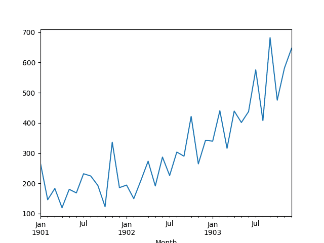
  Line Plot of Shampoo Sales Dataset

  Next, we will take a look at the LSTM configuration and test harness used in the experiment.

  Need help with Deep Learning for Time Series?

  Take my free 7-day email crash course now (with sample code).

  Click to sign-up and also get a free PDF Ebook version of the course.

  LSTM Model and Test Harness

  Data Split

  We will split the Shampoo Sales dataset into two parts: a training and a test set.

  The first two years of data will be taken for the training dataset and the remaining one year of data will be used for the test set.

  Models will be developed using the training dataset and will make predictions on the test dataset.

  Model Evaluation

  A rolling-forecast scenario will be used, also called walk-forward model validation.

  Each time step of the test dataset will be walked one at a time. A model will be used to make a forecast for the time step, then the actual expected value from the test set will be taken and made available to the model for the forecast on the next time step.

  This mimics a real-world scenario where new Shampoo Sales observations would be available each month and used in the forecasting of the following month.

  This will be simulated by the structure of the train and test datasets. We will make all of the forecasts in a one-shot method.

  All forecasts on the test dataset will be collected and an error score calculated to summarize the skill of the model. The root mean squared error (RMSE) will be used as it punishes large errors and results in a score that is in the same units as the forecast data, namely monthly shampoo sales.

  Data Preparation

  Before we can fit an LSTM model to the dataset, we must transform the data.

  The following three data transforms are performed on the dataset prior to fitting a model and making a forecast.

  1. Transform the time series data so that it is stationary. Specifically a lag=1 differencing to remove the increasing trend in the data.
  2. Transform the time series into a supervised learning problem. Specifically the organization of data into input and output patterns where the observation at the previous time step is used as an input to forecast the observation at the current timestep.
  3. Transform the observations to have a specific scale. Specifically, to rescale the data to values between -1 and 1 to meet the default hyperbolic tangent activation function of the LSTM model.

  LSTM Model

  An LSTM model configuration will be used that is skillful but untuned.

  This means that the model will be fit to the data and will be able to make meaningful forecasts, but will not be the optimal model for the dataset.

  The network topology consists of 1 input, a hidden layer with 4 units, and an output layer with 1 output value.

  The model will be fit for 3,000 epochs with a batch size of 4. The training dataset will be reduced to 20 observations after data preparation. This is so that the batch size evenly divides into both the training dataset and the test dataset (a requirement).

  Experimental Run

  Each scenario will be run 30 times.

  This means that 30 models will be created and evaluated for each scenario. The RMSE from each run will be collected providing a population of results that can be summarized using descriptive statistics like the mean and standard deviation.

  This is required because neural networks like the LSTM are influenced by their initial conditions (e.g. their initial random weights).

  The mean results for each scenario will allow us to interpret the average behavior of each scenario and how they compare.

  Let’s dive into the results.

  Code Listing

  Key modular behaviors were separated into functions for readability and testability, in case you would like to reuse this experimental setup.

  The specifics of the scenarios are described in the experiment() function.

  The complete code listing is provided below.

  from pandas import DataFrame from pandas import Series from pandas import concat from pandas import read_csv from pandas import datetime from sklearn.metrics import mean_squared_error from sklearn.preprocessing import MinMaxScaler from keras.models import Sequential from keras.layers import Dense from keras.layers import LSTM from math import sqrt import matplotlib # be able to save images on server matplotlib.use('Agg') from matplotlib import pyplot import numpy   # date-time parsing function for loading the dataset def parser(x): return datetime.strptime('190'+x, '%Y-%m')   # frame a sequence as a supervised learning problem def timeseries_to_supervised(data, lag=1): df = DataFrame(data) columns = [df.shift(i) for i in range(1, lag+1)] columns.append(df) df = concat(columns, axis=1) df = df.drop(0) return df   # create a differenced series def difference(dataset, interval=1): diff = list() for i in range(interval, len(dataset)): value = dataset[i] - dataset[i - interval] diff.append(value) return Series(diff)   # invert differenced value def inverse_difference(history, yhat, interval=1): return yhat + history[-interval]   # scale train and test data to [-1, 1] def scale(train, test): # fit scaler scaler = MinMaxScaler(feature_range=(-1, 1)) scaler = scaler.fit(train) # transform train train = train.reshape(train.shape[0], train.shape[1]) train_scaled = scaler.transform(train) # transform test test = test.reshape(test.shape[0], test.shape[1]) test_scaled = scaler.transform(test) return scaler, train_scaled, test_scaled   # inverse scaling for a forecasted value def invert_scale(scaler, X, yhat): new_row = [x for x in X] + [yhat] array = numpy.array(new_row) array = array.reshape(1, len(array)) inverted = scaler.inverse_transform(array) return inverted[0, -1]   # fit an LSTM network to training data def fit_lstm(train, batch_size, nb_epoch, neurons): X, y = train[:, 0:-1], train[:, -1] X = X.reshape(X.shape[0], 1, X.shape[1]) model = Sequential() model.add(LSTM(neurons, batch_input_shape=(batch_size, X.shape[1], X.shape[2]), stateful=True)) model.add(Dense(1)) model.compile(loss='mean_squared_error', optimizer='adam') for i in range(nb_epoch): model.fit(X, y, epochs=1, batch_size=batch_size, verbose=0, shuffle=False) model.reset_states() return model   # make a one-step forecast def forecast_lstm(model, batch_size, X): X = X.reshape(1, 1, len(X)) yhat = model.predict(X, batch_size=batch_size) return yhat[0,0]   # run a repeated experiment def experiment(repeats, series, seed): # transform data to be stationary raw_values = series.values diff_values = difference(raw_values, 1) # transform data to be supervised learning supervised = timeseries_to_supervised(diff_values, 1) supervised_values = supervised.values # split data into train and test-sets train, test = supervised_values[0:-12], supervised_values[-12:] # transform the scale of the data scaler, train_scaled, test_scaled = scale(train, test) # run experiment error_scores = list() for r in range(repeats): # fit the model batch_size = 4 train_trimmed = train_scaled[2:, :] lstm_model = fit_lstm(train_trimmed, batch_size, 3000, 4) # forecast the entire training dataset to build up state for forecasting if seed: train_reshaped = train_trimmed[:, 0].reshape(len(train_trimmed), 1, 1) lstm_model.predict(train_reshaped, batch_size=batch_size) # forecast test dataset test_reshaped = test_scaled[:,0:-1] test_reshaped = test_reshaped.reshape(len(test_reshaped), 1, 1) output = lstm_model.predict(test_reshaped, batch_size=batch_size) predictions = list() for i in range(len(output)): yhat = output[i,0] X = test_scaled[i, 0:-1] # invert scaling yhat = invert_scale(scaler, X, yhat) # invert differencing yhat = inverse_difference(raw_values, yhat, len(test_scaled)+1-i) # store forecast predictions.append(yhat) # report performance rmse = sqrt(mean_squared_error(raw_values[-12:], predictions)) print('%d) Test RMSE: %.3f' % (r+1, rmse)) error_scores.append(rmse) return error_scores   # load dataset series = read_csv('shampoo-sales.csv', header=0, parse_dates=[0], index_col=0, squeeze=True, date_parser=parser) # experiment repeats = 30 results = DataFrame() # with seeding with_seed = experiment(repeats, series, True) results['with-seed'] = with_seed # without seeding without_seed = experiment(repeats, series, False) results['without-seed'] = without_seed # summarize results print(results.describe()) # save boxplot results.boxplot() pyplot.savefig('boxplot.png')

  Experimental Results

  Running the experiment takes some time or CPU or GPU hardware.

  The RMSE of each run is printed to give an idea of progress.

  At the end of the run, the summary statistics are calculated and printed for each scenario, including the mean and standard deviation.

  Note: Your results may vary given the stochastic nature of the algorithm or evaluation procedure, or differences in numerical precision. Consider running the example a few times and compare the average outcome.

  The complete output is listed below.

  1) Test RMSE: 86.566 2) Test RMSE: 300.874 3) Test RMSE: 169.237 4) Test RMSE: 167.939 5) Test RMSE: 135.416 6) Test RMSE: 291.746 7) Test RMSE: 220.729 8) Test RMSE: 222.815 9) Test RMSE: 236.043 10) Test RMSE: 134.183 11) Test RMSE: 145.320 12) Test RMSE: 142.771 13) Test RMSE: 239.289 14) Test RMSE: 218.629 15) Test RMSE: 208.855 16) Test RMSE: 187.421 17) Test RMSE: 141.151 18) Test RMSE: 174.379 19) Test RMSE: 241.310 20) Test RMSE: 226.963 21) Test RMSE: 126.777 22) Test RMSE: 197.340 23) Test RMSE: 149.662 24) Test RMSE: 235.681 25) Test RMSE: 200.320 26) Test RMSE: 92.396 27) Test RMSE: 169.573 28) Test RMSE: 219.894 29) Test RMSE: 168.048 30) Test RMSE: 141.638 1) Test RMSE: 85.470 2) Test RMSE: 151.935 3) Test RMSE: 102.314 4) Test RMSE: 215.588 5) Test RMSE: 172.948 6) Test RMSE: 114.746 7) Test RMSE: 205.958 8) Test RMSE: 89.335 9) Test RMSE: 183.635 10) Test RMSE: 173.400 11) Test RMSE: 116.645 12) Test RMSE: 133.473 13) Test RMSE: 155.044 14) Test RMSE: 153.582 15) Test RMSE: 146.693 16) Test RMSE: 95.455 17) Test RMSE: 104.970 18) Test RMSE: 127.700 19) Test RMSE: 189.728 20) Test RMSE: 127.756 21) Test RMSE: 102.795 22) Test RMSE: 189.742 23) Test RMSE: 144.621 24) Test RMSE: 132.053 25) Test RMSE: 238.034 26) Test RMSE: 139.800 27) Test RMSE: 202.881 28) Test RMSE: 172.278 29) Test RMSE: 125.565 30) Test RMSE: 103.868         with-seed  without-seed count   30.000000     30.000000 mean   186.432143    146.600505 std     52.559598     40.554595 min     86.565993     85.469737 25%    143.408162    115.221000 50%    180.899814    142.210265 75%    222.293194    173.287017 max    300.873841    238.034137

  A box and whisker plot is also created and saved to file, shown below.

  

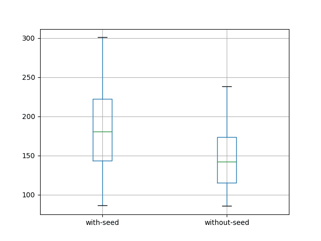
  Box and Whisker Plot of LSTM with and Without Seed of State

  The results are surprising.

  They suggest better results by not seeding the state of the LSTM prior to forecasting the test dataset.

  This can be seen by the lower on average error of 146.600505 monthly shampoo sales compared to 186.432143 with seeding. It is much clearer in the box and whisker plot of the distributions.

  Perhaps the chosen model configuration resulted in a model too small to be dependent on the sequence and internal state to benefit from seeding prior to forecasting. Perhaps larger experiments are required.

  Extensions

  The surprising results open the door to further experimentation.

  • Evaluate the effect of clearing vs not clearing the state after the end of the last training epoch.
  • Evaluate the effect of predicting the training and test sets all at once vs one time step at a time.
  • Evaluate the effect of resetting and not resetting the LSTM state at the end of each epoch.

  Did you try one of these extensions? Share your findings in the comments below.

  Summary

  In this tutorial, you discovered how to experimentally determine the best way to seed the state of an LSTM model on a univariate time series forecasting problem.

  Specifically, you learned:

  • About the problem of seeding the state of an LSTM prior to forecasting and ways to address it.
  • How to develop a robust test harness for evaluating LSTM models for time series forecasting.
  • How to determine whether or not to seed the state of an LSTM model with the training data prior to forecasting.

  Did you run the experiment or run a modified version of the experiment?
  Share your results in the comments; I’d love to see them.

  Do you have any questions about this post?
  Ask your questions in the comment below and I will do my best to answer.