How to Implement Linear Regression From Scratch in Python

 The core of many machine learning algorithms is optimization.

Optimization algorithms are used by machine learning algorithms to find a good set of model parameters given a training dataset.

The most common optimization algorithm used in machine learning is stochastic gradient descent.

In this tutorial, you will discover how to implement stochastic gradient descent to optimize a linear regression algorithm from scratch with Python.

After completing this tutorial, you will know:

• How to estimate linear regression coefficients using stochastic gradient descent.
• How to make predictions for multivariate linear regression.
• How to implement linear regression with stochastic gradient descent to make predictions on new data.

  Description

  In this section, we will describe linear regression, the stochastic gradient descent technique and the wine quality dataset used in this tutorial.

  Multivariate Linear Regression

  Linear regression is a technique for predicting a real value.

  Confusingly, these problems where a real value is to be predicted are called regression problems.

  Linear regression is a technique where a straight line is used to model the relationship between input and output values. In more than two dimensions, this straight line may be thought of as a plane or hyperplane.

  Predictions are made as a combination of the input values to predict the output value.

  Each input attribute (x) is weighted using a coefficient (b), and the goal of the learning algorithm is to discover a set of coefficients that results in good predictions (y).

  y = b0 + b1 * x1 + b2 * x2 + ...

  Coefficients can be found using stochastic gradient descent.

  Stochastic Gradient Descent

  Gradient Descent is the process of minimizing a function by following the gradients of the cost function.

  This involves knowing the form of the cost as well as the derivative so that from a given point you know the gradient and can move in that direction, e.g. downhill towards the minimum value.

  In machine learning, we can use a technique that evaluates and updates the coefficients every iteration called stochastic gradient descent to minimize the error of a model on our training data.

  The way this optimization algorithm works is that each training instance is shown to the model one at a time. The model makes a prediction for a training instance, the error is calculated and the model is updated in order to reduce the error for the next prediction. This process is repeated for a fixed number of iterations.

  This procedure can be used to find the set of coefficients in a model that result in the smallest error for the model on the training data. Each iteration, the coefficients (b) in machine learning language are updated using the equation:

  b = b - learning_rate * error * x

  Where b is the coefficient or weight being optimized, learning_rate is a learning rate that you must configure (e.g. 0.01), error is the prediction error for the model on the training data attributed to the weight, and x is the input value.

  Wine Quality Dataset

  After we develop our linear regression algorithm with stochastic gradient descent, we will use it to model the wine quality dataset.

  This dataset is comprised of the details of 4,898 white wines including measurements like acidity and pH. The goal is to use these objective measures to predict the wine quality on a scale between 0 and 10.

  Below is a sample of the first 5 records from this dataset.

  7,0.27,0.36,20.7,0.045,45,170,1.001,3,0.45,8.8,6 6.3,0.3,0.34,1.6,0.049,14,132,0.994,3.3,0.49,9.5,6 8.1,0.28,0.4,6.9,0.05,30,97,0.9951,3.26,0.44,10.1,6 7.2,0.23,0.32,8.5,0.058,47,186,0.9956,3.19,0.4,9.9,6 7.2,0.23,0.32,8.5,0.058,47,186,0.9956,3.19,0.4,9.9,6

  The dataset must be normalized to the values between 0 and 1 as each attribute has different units and in turn different scales.

  By predicting the mean value (Zero Rule Algorithm) on the normalized dataset, a baseline root mean squared error (RMSE) of 0.148 can be achieved.

  You can learn more about the dataset on the UCI Machine Learning Repository.

  You can download the dataset and save it in your current working directory with the name winequality-white.csv. You must remove the header information from the start of the file, and convert the “;” value separator to “,” to meet CSV format.

  Tutorial

  This tutorial is broken down into 3 parts:

  1. Making Predictions.
  2. Estimating Coefficients.
  3. Wine Quality Prediction.

  This will provide the foundation you need to implement and apply linear regression with stochastic gradient descent on your own predictive modeling problems.

  1. Making Predictions

  The first step is to develop a function that can make predictions.

  This will be needed both in the evaluation of candidate coefficient values in stochastic gradient descent and after the model is finalized and we wish to start making predictions on test data or new data.

  Below is a function named predict() that predicts an output value for a row given a set of coefficients.

  The first coefficient in is always the intercept, also called the bias or b0 as it is standalone and not responsible for a specific input value.

  # Make a prediction with coefficients def predict(row, coefficients): yhat = coefficients[0] for i in range(len(row)-1): yhat += coefficients[i + 1] * row[i] return yhat

  We can contrive a small dataset to test our prediction function.

  x, y 1, 1 2, 3 4, 3 3, 2 5, 5

  Below is a plot of this dataset.

  

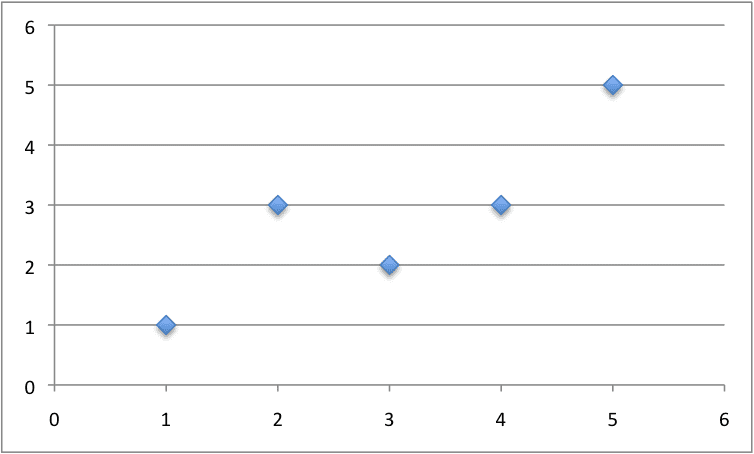
  Small Contrived Dataset For Linear Regression

  We can also use previously prepared coefficients to make predictions for this dataset.

  Putting this all together we can test our predict() function below.

  # Make a prediction with coefficients def predict(row, coefficients): yhat = coefficients[0] for i in range(len(row)-1): yhat += coefficients[i + 1] * row[i] return yhat   dataset = [[1, 1], [2, 3], [4, 3], [3, 2], [5, 5]] coef = [0.4, 0.8] for row in dataset: yhat = predict(row, coef) print("Expected=%.3f, Predicted=%.3f" % (row[-1], yhat))

  There is a single input value (x) and two coefficient values (b0 and b1). The prediction equation we have modeled for this problem is:

  y = b0 + b1 * x

  or, with the specific coefficient values we chose by hand as:

  y = 0.4 + 0.8 * x

  Running this function we get predictions that are reasonably close to the expected output (y) values.

  Expected=1.000, Predicted=1.200 Expected=3.000, Predicted=2.000 Expected=3.000, Predicted=3.600 Expected=2.000, Predicted=2.800 Expected=5.000, Predicted=4.400

  Now we are ready to implement stochastic gradient descent to optimize our coefficient values.

  2. Estimating Coefficients

  We can estimate the coefficient values for our training data using stochastic gradient descent.

  Stochastic gradient descent requires two parameters:

  • Learning Rate: Used to limit the amount each coefficient is corrected each time it is updated.
  • Epochs: The number of times to run through the training data while updating the coefficients.

  These, along with the training data will be the arguments to the function.

  There are 3 loops we need to perform in the function:

  1. Loop over each epoch.
  2. Loop over each row in the training data for an epoch.
  3. Loop over each coefficient and update it for a row in an epoch.

  As you can see, we update each coefficient for each row in the training data, each epoch.

  Coefficients are updated based on the error the model made. The error is calculated as the difference between the prediction made with the candidate coefficients and the expected output value.

  error = prediction - expected

  There is one coefficient to weight each input attribute, and these are updated in a consistent way, for example:

  b1(t+1) = b1(t) - learning_rate * error(t) * x1(t)

  The special coefficient at the beginning of the list, also called the intercept or the bias, is updated in a similar way, except without an input as it is not associated with a specific input value:

  b0(t+1) = b0(t) - learning_rate * error(t)

  Now we can put all of this together. Below is a function named coefficients_sgd() that calculates coefficient values for a training dataset using stochastic gradient descent.

  # Estimate linear regression coefficients using stochastic gradient descent def coefficients_sgd(train, l_rate, n_epoch): coef = [0.0 for i in range(len(train[0]))] for epoch in range(n_epoch): sum_error = 0 for row in train: yhat = predict(row, coef) error = yhat - row[-1] sum_error += error**2 coef[0] = coef[0] - l_rate * error for i in range(len(row)-1): coef[i + 1] = coef[i + 1] - l_rate * error * row[i] print('>epoch=%d, lrate=%.3f, error=%.3f' % (epoch, l_rate, sum_error)) return coef

  You can see, that in addition, we keep track of the sum of the squared error (a positive value) each epoch so that we can print out a nice message in the outer loop.

  We can test this function on the same small contrived dataset from above.

  # Make a prediction with coefficients def predict(row, coefficients): yhat = coefficients[0] for i in range(len(row)-1): yhat += coefficients[i + 1] * row[i] return yhat   # Estimate linear regression coefficients using stochastic gradient descent def coefficients_sgd(train, l_rate, n_epoch): coef = [0.0 for i in range(len(train[0]))] for epoch in range(n_epoch): sum_error = 0 for row in train: yhat = predict(row, coef) error = yhat - row[-1] sum_error += error**2 coef[0] = coef[0] - l_rate * error for i in range(len(row)-1): coef[i + 1] = coef[i + 1] - l_rate * error * row[i] print('>epoch=%d, lrate=%.3f, error=%.3f' % (epoch, l_rate, sum_error)) return coef   # Calculate coefficients dataset = [[1, 1], [2, 3], [4, 3], [3, 2], [5, 5]] l_rate = 0.001 n_epoch = 50 coef = coefficients_sgd(dataset, l_rate, n_epoch) print(coef)

  We use a small learning rate of 0.001 and train the model for 50 epochs, or 50 exposures of the coefficients to the entire training dataset.

  Running the example prints a message each epoch with the sum squared error for that epoch and the final set of coefficients.

  >epoch=45, lrate=0.001, error=2.650 >epoch=46, lrate=0.001, error=2.627 >epoch=47, lrate=0.001, error=2.607 >epoch=48, lrate=0.001, error=2.589 >epoch=49, lrate=0.001, error=2.573 [0.22998234937311363, 0.8017220304137576]

  You can see how error continues to drop even in the final epoch. We could probably train for a lot longer (more epochs) or increase the amount we update the coefficients each epoch (higher learning rate).

  Experiment and see what you come up with.

  Now, let’s apply this algorithm on a real dataset.

  3. Wine Quality Prediction

  In this section, we will train a linear regression model using stochastic gradient descent on the wine quality dataset.

  The example assumes that a CSV copy of the dataset is in the current working directory with the filename winequality-white.csv.

  The dataset is first loaded, the string values converted to numeric and each column is normalized to values in the range of 0 to 1. This is achieved with helper functions load_csv() and str_column_to_float() to load and prepare the dataset and dataset_minmax() and normalize_dataset() to normalize it.

  We will use k-fold cross-validation to estimate the performance of the learned model on unseen data. This means that we will construct and evaluate k models and estimate the performance as the mean model error. Root mean squared error will be used to evaluate each model. These behaviors are provided in the cross_validation_split(), rmse_metric() and evaluate_algorithm() helper functions.

  We will use the predict(), coefficients_sgd() and linear_regression_sgd() functions created above to train the model.

  Below is the complete example.

  # Linear Regression With Stochastic Gradient Descent for Wine Quality from random import seed from random import randrange from csv import reader from math import sqrt   # Load a CSV file def load_csv(filename): dataset = list() with open(filename, 'r') as file: csv_reader = reader(file) for row in csv_reader: if not row: continue dataset.append(row) return dataset   # Convert string column to float def str_column_to_float(dataset, column): for row in dataset: row[column] = float(row[column].strip())   # Find the min and max values for each column def dataset_minmax(dataset): minmax = list() for i in range(len(dataset[0])): col_values = [row[i] for row in dataset] value_min = min(col_values) value_max = max(col_values) minmax.append([value_min, value_max]) return minmax   # Rescale dataset columns to the range 0-1 def normalize_dataset(dataset, minmax): for row in dataset: for i in range(len(row)): row[i] = (row[i] - minmax[i][0]) / (minmax[i][1] - minmax[i][0])   # Split a dataset into k folds def cross_validation_split(dataset, n_folds): dataset_split = list() dataset_copy = list(dataset) fold_size = int(len(dataset) / n_folds) for i in range(n_folds): fold = list() while len(fold) < fold_size: index = randrange(len(dataset_copy)) fold.append(dataset_copy.pop(index)) dataset_split.append(fold) return dataset_split   # Calculate root mean squared error def rmse_metric(actual, predicted): sum_error = 0.0 for i in range(len(actual)): prediction_error = predicted[i] - actual[i] sum_error += (prediction_error ** 2) mean_error = sum_error / float(len(actual)) return sqrt(mean_error)   # Evaluate an algorithm using a cross validation split def evaluate_algorithm(dataset, algorithm, n_folds, *args): folds = cross_validation_split(dataset, n_folds) scores = list() for fold in folds: train_set = list(folds) train_set.remove(fold) train_set = sum(train_set, []) test_set = list() for row in fold: row_copy = list(row) test_set.append(row_copy) row_copy[-1] = None predicted = algorithm(train_set, test_set, *args) actual = [row[-1] for row in fold] rmse = rmse_metric(actual, predicted) scores.append(rmse) return scores   # Make a prediction with coefficients def predict(row, coefficients): yhat = coefficients[0] for i in range(len(row)-1): yhat += coefficients[i + 1] * row[i] return yhat   # Estimate linear regression coefficients using stochastic gradient descent def coefficients_sgd(train, l_rate, n_epoch): coef = [0.0 for i in range(len(train[0]))] for epoch in range(n_epoch): for row in train: yhat = predict(row, coef) error = yhat - row[-1] coef[0] = coef[0] - l_rate * error for i in range(len(row)-1): coef[i + 1] = coef[i + 1] - l_rate * error * row[i] # print(l_rate, n_epoch, error) return coef   # Linear Regression Algorithm With Stochastic Gradient Descent def linear_regression_sgd(train, test, l_rate, n_epoch): predictions = list() coef = coefficients_sgd(train, l_rate, n_epoch) for row in test: yhat = predict(row, coef) predictions.append(yhat) return(predictions)   # Linear Regression on wine quality dataset seed(1) # load and prepare data filename = 'winequality-white.csv' dataset = load_csv(filename) for i in range(len(dataset[0])): str_column_to_float(dataset, i) # normalize minmax = dataset_minmax(dataset) normalize_dataset(dataset, minmax) # evaluate algorithm n_folds = 5 l_rate = 0.01 n_epoch = 50 scores = evaluate_algorithm(dataset, linear_regression_sgd, n_folds, l_rate, n_epoch) print('Scores: %s' % scores) print('Mean RMSE: %.3f' % (sum(scores)/float(len(scores))))

  A k value of 5 was used for cross-validation, giving each fold 4,898/5 = 979.6 or just under 1000 records to be evaluated upon each iteration. A learning rate of 0.01 and 50 training epochs were chosen with a little experimentation.

  You can try your own configurations and see if you can beat my score.

  Running this example prints the scores for each of the 5 cross-validation folds then prints the mean RMSE.

  We can see that the RMSE (on the normalized dataset) is 0.126, lower than the baseline value of 0.148 if we just predicted the mean (using the Zero Rule Algorithm).

  Scores: [0.12248058224159092, 0.13034017509167112, 0.12620370547483578, 0.12897687952843237, 0.12446990678682233] Mean RMSE: 0.126

  Extensions

  This section lists a number of extensions to this tutorial that you may wish to consider exploring.

  • Tune The Example. Tune the learning rate, number of epochs and even the data preparation method to get an improved score on the wine quality dataset.
  • Batch Stochastic Gradient Descent. Change the stochastic gradient descent algorithm to accumulate updates across each epoch and only update the coefficients in a batch at the end of the epoch.
  • Additional Regression Problems. Apply the technique to other regression problems on the UCI machine learning repository.

  Did you explore any of these extensions?
  Let me know about it in the comments below.

  Review

  In this tutorial, you discovered how to implement linear regression using stochastic gradient descent from scratch with Python.

  You learned.

  • How to make predictions for a multivariate linear regression problem.
  • How to optimize a set of coefficients using stochastic gradient descent.
  • How to apply the technique to a real regression predictive modeling problem.