How to implement a close to state-of-the-art deep learning model for MNISTDescription of the MNIST Handwritten Digit Recognition Problem
The MNIST problem
is a dataset developed by Yann LeCun, Corinna Cortes, and Christopher
Burges for evaluating machine learning models on the handwritten digit
classification problem.
The dataset was constructed from a number of scanned document datasets available from the National Institute of Standards and Technology (NIST). This is where the name for the dataset comes from, the Modified NIST or MNIST dataset.
Images of digits were taken from a variety of scanned documents,
normalized in size, and centered. This makes it an excellent dataset for
evaluating models, allowing the developer to focus on machine learning
with minimal data cleaning or preparation required.
Each image is a 28×28-pixel square (784 pixels total). A standard
split of the dataset is used to evaluate and compare models, where
60,000 images are used to train a model, and a separate set of 10,000
images are used to test it.
It is a digit recognition task. As such, there are ten digits (0 to
9) or ten classes to predict. Results are reported using prediction
error, which is nothing more than the inverted classification accuracy.
Excellent results achieve a prediction error of less than 1%. A
state-of-the-art prediction error of approximately 0.2% can be achieved
with large convolutional neural networks. There is a listing of the
state-of-the-art results and links to the relevant papers on the MNIST
and other datasets on Rodrigo Benenson’s webpage.
Need help with Deep Learning in Python?
Take my free 2-week email course and discover MLPs, CNNs and LSTMs (with code).
Click to sign-up now and also get a free PDF Ebook version of the course.
Loading the MNIST Dataset in Keras
The Keras deep learning library provides a convenient method for loading the MNIST dataset.
The dataset is downloaded automatically the first time this function is called and stored in your home directory in ~/.keras/datasets/mnist.npz as an 11MB file.
This is very handy for developing and testing deep learning models.
To demonstrate how easy it is to load the MNIST dataset, first, write
a little script to download and visualize the first four images in the
training dataset.
# Plot ad hoc mnist instances from tensorflow.keras.datasets import mnist import matplotlib.pyplot as plt # load (downloaded if needed) the MNIST dataset (X_train, y_train), (X_test, y_test) = mnist.load_data() # plot 4 images as gray scale plt.subplot(221) plt.imshow(X_train[0], cmap=plt.get_cmap('gray')) plt.subplot(222) plt.imshow(X_train[1], cmap=plt.get_cmap('gray')) plt.subplot(223) plt.imshow(X_train[2], cmap=plt.get_cmap('gray')) plt.subplot(224) plt.imshow(X_train[3], cmap=plt.get_cmap('gray')) # show the plot plt.show() |
You can see that downloading and loading the MNIST dataset is
as easy as calling the mnist.load_data() function. Running the above
example, you should see the image below.
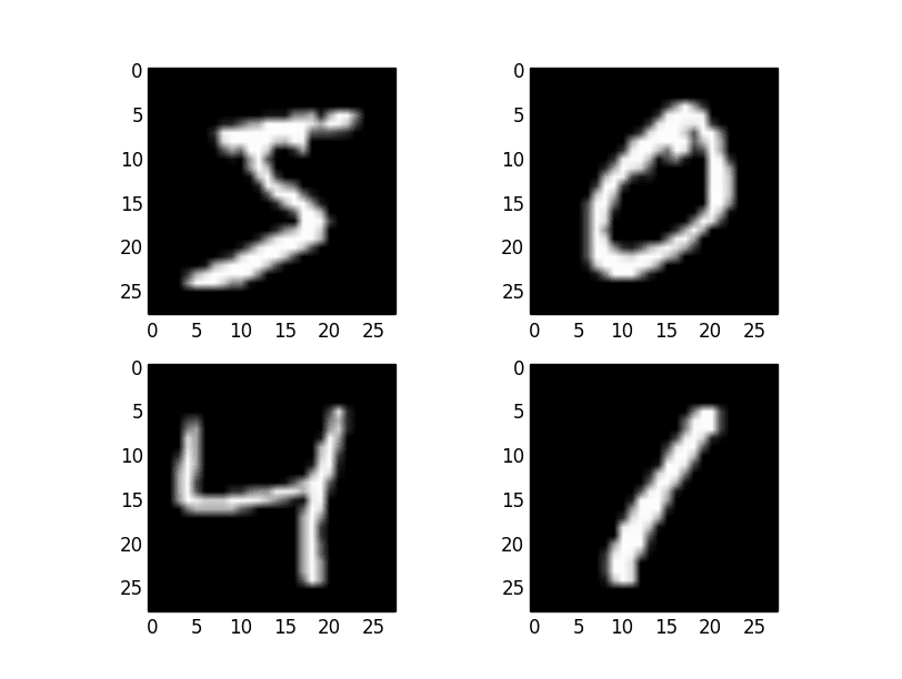
Examples from the MNIST dataset
Baseline Model with Multi-Layer Perceptrons
Do you really need a complex model like a convolutional neural network to get the best results with MNIST?
You can get very good results using a very simple neural network
model with a single hidden layer. In this section, you will create a
simple multi-layer perceptron model that achieves an error rate of
1.74%. You will use this as a baseline for comparing more complex
convolutional neural network models.
Let’s start by importing the classes and functions you will need.
from tensorflow.keras.datasets import mnist from tensorflow.keras.models import Sequential from tensorflow.keras.layers import Dense from tensorflow.keras.layers import Dropout from tensorflow.keras.utils import to_categorical ... |
Now, you can load the MNIST dataset using the Keras helper function.
... # load data (X_train, y_train), (X_test, y_test) = mnist.load_data() |
The training dataset is structured as a 3-dimensional array of
instance, image width, and image height. For a multi-layer perceptron
model, you must reduce the images down into a vector of pixels. In this
case, the 28×28-sized images will be 784 pixel input values.
You can do this transform easily using the reshape() function
on the NumPy array. You can also reduce your memory requirements by
forcing the precision of the pixel values to be 32-bit, the default
precision used by Keras anyway.
... # flatten 28*28 images to a 784 vector for each image num_pixels = X_train.shape[1] * X_train.shape[2] X_train = X_train.reshape((X_train.shape[0], num_pixels)).astype('float32') X_test = X_test.reshape((X_test.shape[0], num_pixels)).astype('float32') |
The pixel values are grayscale between 0 and 255. It is almost
always a good idea to perform some scaling of input values when using
neural network models. Because the scale is well known and well behaved,
you can very quickly normalize the pixel values to the range 0 and 1 by
dividing each value by the maximum of 255.
... # normalize inputs from 0-255 to 0-1 X_train = X_train / 255 X_test = X_test / 255 |
Finally, the output variable is an integer from 0 to 9. This is
a multi-class classification problem. As such, it is good practice to
use a one-hot encoding of the class values, transforming the vector of
class integers into a binary matrix.
You can easily do this using the built-in tf.keras.utils.to_categorical() helper function in Keras.
... # one hot encode outputs y_train = to_categorical(y_train) y_test = to_categorical(y_test) num_classes = y_test.shape[1] |
You are now ready to create your simple neural network model.
You will define your model in a function. This is handy if you want to
extend the example later and try and get a better score.
... # define baseline model def baseline_model(): # create model model = Sequential() model.add(Dense(num_pixels, input_shape=(num_pixels,), kernel_initializer='normal', activation='relu')) model.add(Dense(num_classes, kernel_initializer='normal', activation='softmax')) # Compile model model.compile(loss='categorical_crossentropy', optimizer='adam', metrics=['accuracy']) return model |
The model is a simple neural network with one hidden layer with
the same number of neurons as there are inputs (784). A rectifier
activation function is used for the neurons in the hidden layer.
A softmax activation function is used on the output layer to turn the
outputs into probability-like values and allow one class of the ten to
be selected as the model’s output prediction. Logarithmic loss is used
as the loss function (called categorical_crossentropy in Keras), and the
efficient ADAM gradient descent algorithm is used to learn the weights.
You can now fit and evaluate the model. The model is fit over ten
epochs with updates every 200 images. The test data is used as the
validation dataset, allowing you to see the skill of the model as it
trains. A verbose value of 2 is used to reduce the output to one line
for each training epoch.
Finally, the test dataset is used to evaluate the model, and a classification error rate is printed.
... # build the model model = baseline_model() # Fit the model model.fit(X_train, y_train, validation_data=(X_test, y_test), epochs=10, batch_size=200, verbose=2) # Final evaluation of the model scores = model.evaluate(X_test, y_test, verbose=0) print("Baseline Error: %.2f%%" % (100-scores[1]*100)) |
After tying this all together, the complete code listing is provided below.
# Baseline MLP for MNIST dataset from tensorflow.keras.datasets import mnist from tensorflow.keras.models import Sequential from tensorflow.keras.layers import Dense from tensorflow.keras.utils import to_categorical # load data (X_train, y_train), (X_test, y_test) = mnist.load_data() # flatten 28*28 images to a 784 vector for each image num_pixels = X_train.shape[1] * X_train.shape[2] X_train = X_train.reshape((X_train.shape[0], num_pixels)).astype('float32') X_test = X_test.reshape((X_test.shape[0], num_pixels)).astype('float32') # normalize inputs from 0-255 to 0-1 X_train = X_train / 255 X_test = X_test / 255 # one hot encode outputs y_train = to_categorical(y_train) y_test = to_categorical(y_test) num_classes = y_test.shape[1] # define baseline model def baseline_model(): # create model model = Sequential() model.add(Dense(num_pixels, input_shape=(num_pixels,), kernel_initializer='normal', activation='relu')) model.add(Dense(num_classes, kernel_initializer='normal', activation='softmax')) # Compile model model.compile(loss='categorical_crossentropy', optimizer='adam', metrics=['accuracy']) return model # build the model model = baseline_model() # Fit the model model.fit(X_train, y_train, validation_data=(X_test, y_test), epochs=10, batch_size=200, verbose=2) # Final evaluation of the model scores = model.evaluate(X_test, y_test, verbose=0) print("Baseline Error: %.2f%%" % (100-scores[1]*100)) |
Running the example might take a few minutes when you run it on a CPU.
Note: Your results may vary
given the stochastic nature of the algorithm or evaluation procedure,
or differences in numerical precision. Consider running the example a
few times and compare the average outcome.
You should see the output below. This very simple network defined in
very few lines of code achieves a respectable error rate of 2.3%.
Epoch 1/10 300/300 - 1s - loss: 0.2792 - accuracy: 0.9215 - val_loss: 0.1387 - val_accuracy: 0.9590 - 1s/epoch - 4ms/step Epoch 2/10 300/300 - 1s - loss: 0.1113 - accuracy: 0.9676 - val_loss: 0.0923 - val_accuracy: 0.9709 - 929ms/epoch - 3ms/step Epoch 3/10 300/300 - 1s - loss: 0.0704 - accuracy: 0.9799 - val_loss: 0.0728 - val_accuracy: 0.9787 - 912ms/epoch - 3ms/step Epoch 4/10 300/300 - 1s - loss: 0.0502 - accuracy: 0.9859 - val_loss: 0.0664 - val_accuracy: 0.9808 - 904ms/epoch - 3ms/step Epoch 5/10 300/300 - 1s - loss: 0.0356 - accuracy: 0.9897 - val_loss: 0.0636 - val_accuracy: 0.9803 - 905ms/epoch - 3ms/step Epoch 6/10 300/300 - 1s - loss: 0.0261 - accuracy: 0.9932 - val_loss: 0.0591 - val_accuracy: 0.9813 - 907ms/epoch - 3ms/step Epoch 7/10 300/300 - 1s - loss: 0.0195 - accuracy: 0.9953 - val_loss: 0.0564 - val_accuracy: 0.9828 - 910ms/epoch - 3ms/step Epoch 8/10 300/300 - 1s - loss: 0.0145 - accuracy: 0.9969 - val_loss: 0.0580 - val_accuracy: 0.9810 - 954ms/epoch - 3ms/step Epoch 9/10 300/300 - 1s - loss: 0.0116 - accuracy: 0.9973 - val_loss: 0.0594 - val_accuracy: 0.9817 - 947ms/epoch - 3ms/step Epoch 10/10 300/300 - 1s - loss: 0.0079 - accuracy: 0.9985 - val_loss: 0.0735 - val_accuracy: 0.9770 - 914ms/epoch - 3ms/step Baseline Error: 2.30% |
Simple Convolutional Neural Network for MNIST
Now that you have seen how to load the MNIST dataset and train a
simple multi-layer perceptron model on it, it is time to develop a more
sophisticated convolutional neural network or CNN model.
Keras does provide a lot of capability for creating convolutional neural networks.
In this section, you will create a simple CNN for MNIST that
demonstrates how to use all the aspects of a modern CNN implementation,
including Convolutional layers, Pooling layers, and Dropout layers.
The first step is to import the classes and functions needed.
from tensorflow.keras.datasets import mnist from tensorflow.keras.models import Sequential from tensorflow.keras.layers import Dense from tensorflow.keras.layers import Dropout from tensorflow.keras.layers import Flatten from tensorflow.keras.layers import Conv2D from tensorflow.keras.layers import MaxPooling2D from tensorflow.keras.utils import to_categorical ... |
Next, you need to load the MNIST dataset and reshape it to be
suitable for training a CNN. In Keras, the layers used for
two-dimensional convolutions expect pixel values with the dimensions
[pixels][width][height][channels].
Note that you are forcing so-called channels-last ordering for consistency in this example.
In the case of RGB, the last dimension pixels would be 3 for the red,
green, and blue components, and it would be like having three image
inputs for every color image. In the case of MNIST, where the pixel
values are grayscale, the pixel dimension is set to 1.
... # load data (X_train, y_train), (X_test, y_test) = mnist.load_data() # reshape to be [samples][width][height][channels] X_train = X_train.reshape(X_train.shape[0], 28, 28, 1).astype('float32') X_test = X_test.reshape(X_test.shape[0], 28, 28, 1).astype('float32') |
As before, it is a good idea to normalize the pixel values to the range 0 and 1 and one-hot encode the output variables.
... # normalize inputs from 0-255 to 0-1 X_train = X_train / 255 X_test = X_test / 255 # one hot encode outputs y_train = to_categorical(y_train) y_test = to_categorical(y_test) num_classes = y_test.shape[1] |
Next, define your neural network model.
Convolutional neural networks are more complex than standard
multi-layer perceptrons, so you will start by using a simple structure
that uses all the elements for state-of-the-art results. Below
summarizes the network architecture.
- The first hidden layer is a convolutional layer called a
Convolution2D. The layer has 32 feature maps, with the size of 5×5 and a
rectifier activation function. This is the input layer that expects
images with the structure outlined above: [pixels][width][height].
- Next, define a pooling layer that takes the max called MaxPooling2D. It is configured with a pool size of 2×2.
- The next layer is a regularization layer using dropout called
Dropout. It is configured to randomly exclude 20% of neurons in the
layer in order to reduce overfitting.
- Next is a layer that converts the 2D matrix data to a vector called
Flatten. It allows the output to be processed by standard, fully
connected layers.
- Next is a fully connected layer with 128 neurons and a rectifier activation function.
- Finally, the output layer has ten neurons for the ten classes and a
softmax activation function to output probability-like predictions for
each class.
As before, the model is trained using logarithmic loss and the ADAM gradient descent algorithm.
... def baseline_model(): # create model model = Sequential() model.add(Conv2D(32, (5, 5), input_shape=(28, 28, 1), activation='relu')) model.add(MaxPooling2D(pool_size=(2, 2))) model.add(Dropout(0.2)) model.add(Flatten()) model.add(Dense(128, activation='relu')) model.add(Dense(num_classes, activation='softmax')) # Compile model model.compile(loss='categorical_crossentropy', optimizer='adam', metrics=['accuracy']) return model |
You evaluate the model the same way as before with the
multi-layer perceptron. The CNN is fit over ten epochs with a batch size
of 200.
... # build the model model = baseline_model() # Fit the model model.fit(X_train, y_train, validation_data=(X_test, y_test), epochs=10, batch_size=200, verbose=2) # Final evaluation of the model scores = model.evaluate(X_test, y_test, verbose=0) print("CNN Error: %.2f%%" % (100-scores[1]*100)) |
After tying this all together, the complete example is listed below.
# Simple CNN for the MNIST Dataset from tensorflow.keras.datasets import mnist from tensorflow.keras.models import Sequential from tensorflow.keras.layers import Dense from tensorflow.keras.layers import Dropout from tensorflow.keras.layers import Flatten from tensorflow.keras.layers import Conv2D from tensorflow.keras.layers import MaxPooling2D from tensorflow.keras.utils import to_categorical # load data (X_train, y_train), (X_test, y_test) = mnist.load_data() # reshape to be [samples][width][height][channels] X_train = X_train.reshape((X_train.shape[0], 28, 28, 1)).astype('float32') X_test = X_test.reshape((X_test.shape[0], 28, 28, 1)).astype('float32') # normalize inputs from 0-255 to 0-1 X_train = X_train / 255 X_test = X_test / 255 # one hot encode outputs y_train = to_categorical(y_train) y_test = to_categorical(y_test) num_classes = y_test.shape[1] # define a simple CNN model def baseline_model(): # create model model = Sequential() model.add(Conv2D(32, (5, 5), input_shape=(28, 28, 1), activation='relu')) model.add(MaxPooling2D()) model.add(Dropout(0.2)) model.add(Flatten()) model.add(Dense(128, activation='relu')) model.add(Dense(num_classes, activation='softmax')) # Compile model model.compile(loss='categorical_crossentropy', optimizer='adam', metrics=['accuracy']) return model # build the model model = baseline_model() # Fit the model model.fit(X_train, y_train, validation_data=(X_test, y_test), epochs=10, batch_size=200) # Final evaluation of the model scores = model.evaluate(X_test, y_test, verbose=0) print("CNN Error: %.2f%%" % (100-scores[1]*100)) |
After running the example, the accuracy of the training and
validation test is printed for each epoch, and at the end, the
classification error rate is printed.
Note: Your results may vary
given the stochastic nature of the algorithm or evaluation procedure,
or differences in numerical precision. Consider running the example a
few times and compare the average outcome.
Epochs may take about 45 seconds to run on the GPU (e.g., on AWS).
You can see that the network achieves an error rate of 1.19%, which is
better than our simple multi-layer perceptron model above.
Epoch 1/10 300/300 [==============================] - 4s 12ms/step - loss: 0.2372 - accuracy: 0.9344 - val_loss: 0.0715 - val_accuracy: 0.9787 Epoch 2/10 300/300 [==============================] - 4s 13ms/step - loss: 0.0697 - accuracy: 0.9786 - val_loss: 0.0461 - val_accuracy: 0.9858 Epoch 3/10 300/300 [==============================] - 4s 13ms/step - loss: 0.0483 - accuracy: 0.9854 - val_loss: 0.0392 - val_accuracy: 0.9867 Epoch 4/10 300/300 [==============================] - 4s 13ms/step - loss: 0.0366 - accuracy: 0.9887 - val_loss: 0.0357 - val_accuracy: 0.9889 Epoch 5/10 300/300 [==============================] - 4s 14ms/step - loss: 0.0300 - accuracy: 0.9909 - val_loss: 0.0360 - val_accuracy: 0.9873 Epoch 6/10 300/300 [==============================] - 4s 14ms/step - loss: 0.0241 - accuracy: 0.9927 - val_loss: 0.0325 - val_accuracy: 0.9890 Epoch 7/10 300/300 [==============================] - 4s 14ms/step - loss: 0.0210 - accuracy: 0.9932 - val_loss: 0.0314 - val_accuracy: 0.9898 Epoch 8/10 300/300 [==============================] - 4s 14ms/step - loss: 0.0167 - accuracy: 0.9945 - val_loss: 0.0306 - val_accuracy: 0.9898 Epoch 9/10 300/300 [==============================] - 4s 14ms/step - loss: 0.0142 - accuracy: 0.9956 - val_loss: 0.0326 - val_accuracy: 0.9892 Epoch 10/10 300/300 [==============================] - 4s 14ms/step - loss: 0.0114 - accuracy: 0.9966 - val_loss: 0.0322 - val_accuracy: 0.9881 CNN Error: 1.19% |
Larger Convolutional Neural Network for MNIST
Now that you have seen how to create a simple CNN, let’s take a look at a model capable of close to state-of-the-art results.
You will import the classes and functions, then load and prepare the data the same as in the previous CNN example.
# Larger CNN for the MNIST Dataset from tensorflow.keras.datasets import mnist from tensorflow.keras.models import Sequential from tensorflow.keras.layers import Dense from tensorflow.keras.layers import Dropout from tensorflow.keras.layers import Flatten from tensorflow.keras.layers import Conv2D from tensorflow.keras.layers import MaxPooling2D from tensorflow.keras.utils import to_categorical # load data (X_train, y_train), (X_test, y_test) = mnist.load_data() # reshape to be [samples][width][height][channels] X_train = X_train.reshape((X_train.shape[0], 28, 28, 1)).astype('float32') X_test = X_test.reshape((X_test.shape[0], 28, 28, 1)).astype('float32') # normalize inputs from 0-255 to 0-1 X_train = X_train / 255 X_test = X_test / 255 # one hot encode outputs y_train = to_categorical(y_train) y_test = to_categorical(y_test) num_classes = y_test.shape[1] ... |
This time you will define a large CNN architecture with
additional convolutional, max pooling layers, and fully connected
layers. The network topology can be summarized as follows:
- Convolutional layer with 30 feature maps of size 5×5
- Pooling layer taking the max over 2*2 patches
- Convolutional layer with 15 feature maps of size 3×3
- Pooling layer taking the max over 2*2 patches
- Dropout layer with a probability of 20%
- Flatten layer
- Fully connected layer with 128 neurons and rectifier activation
- Fully connected layer with 50 neurons and rectifier activation
- Output layer
... # define the larger model def larger_model(): # create model model = Sequential() model.add(Conv2D(30, (5, 5), input_shape=(28, 28, 1), activation='relu')) model.add(MaxPooling2D(pool_size=(2, 2))) model.add(Conv2D(15, (3, 3), activation='relu')) model.add(MaxPooling2D(pool_size=(2, 2))) model.add(Dropout(0.2)) model.add(Flatten()) model.add(Dense(128, activation='relu')) model.add(Dense(50, activation='relu')) model.add(Dense(num_classes, activation='softmax')) # Compile model model.compile(loss='categorical_crossentropy', optimizer='adam', metrics=['accuracy']) return model |
Like the previous two experiments, the model is fit over ten epochs with a batch size of 200.
... # build the model model = larger_model() # Fit the model model.fit(X_train, y_train, validation_data=(X_test, y_test), epochs=10, batch_size=200) # Final evaluation of the model scores = model.evaluate(X_test, y_test, verbose=0) print("Large CNN Error: %.2f%%" % (100-scores[1]*100)) |
After tying this all together, the complete example is listed below.
# Larger CNN for the MNIST Dataset from tensorflow.keras.datasets import mnist from tensorflow.keras.models import Sequential from tensorflow.keras.layers import Dense from tensorflow.keras.layers import Dropout from tensorflow.keras.layers import Flatten from tensorflow.keras.layers import Conv2D from tensorflow.keras.layers import MaxPooling2D from tensorflow.keras.utils import to_categorical # load data (X_train, y_train), (X_test, y_test) = mnist.load_data() # reshape to be [samples][width][height][channels] X_train = X_train.reshape((X_train.shape[0], 28, 28, 1)).astype('float32') X_test = X_test.reshape((X_test.shape[0], 28, 28, 1)).astype('float32') # normalize inputs from 0-255 to 0-1 X_train = X_train / 255 X_test = X_test / 255 # one hot encode outputs y_train = to_categorical(y_train) y_test = to_categorical(y_test) num_classes = y_test.shape[1] # define the larger model def larger_model(): # create model model = Sequential() model.add(Conv2D(30, (5, 5), input_shape=(28, 28, 1), activation='relu')) model.add(MaxPooling2D()) model.add(Conv2D(15, (3, 3), activation='relu')) model.add(MaxPooling2D()) model.add(Dropout(0.2)) model.add(Flatten()) model.add(Dense(128, activation='relu')) model.add(Dense(50, activation='relu')) model.add(Dense(num_classes, activation='softmax')) # Compile model model.compile(loss='categorical_crossentropy', optimizer='adam', metrics=['accuracy']) return model # build the model model = larger_model() # Fit the model model.fit(X_train, y_train, validation_data=(X_test, y_test), epochs=10, batch_size=200) # Final evaluation of the model scores = model.evaluate(X_test, y_test, verbose=0) print("Large CNN Error: %.2f%%" % (100-scores[1]*100)) |
Running the example prints accuracy on the training and validation datasets of each epoch and a final classification error rate.
Note: Your results may vary
given the stochastic nature of the algorithm or evaluation procedure,
or differences in numerical precision. Consider running the example a
few times and compare the average outcome.
The model takes about 100 seconds to run per epoch. This slightly
larger model achieves a respectable classification error rate of 0.83%.
Epoch 1/10 300/300 [==============================] - 4s 14ms/step - loss: 0.4104 - accuracy: 0.8727 - val_loss: 0.0870 - val_accuracy: 0.9732 Epoch 2/10 300/300 [==============================] - 5s 15ms/step - loss: 0.1062 - accuracy: 0.9669 - val_loss: 0.0601 - val_accuracy: 0.9804 Epoch 3/10 300/300 [==============================] - 4s 14ms/step - loss: 0.0771 - accuracy: 0.9765 - val_loss: 0.0555 - val_accuracy: 0.9803 Epoch 4/10 300/300 [==============================] - 4s 14ms/step - loss: 0.0624 - accuracy: 0.9812 - val_loss: 0.0393 - val_accuracy: 0.9878 Epoch 5/10 300/300 [==============================] - 4s 15ms/step - loss: 0.0521 - accuracy: 0.9838 - val_loss: 0.0333 - val_accuracy: 0.9892 Epoch 6/10 300/300 [==============================] - 4s 15ms/step - loss: 0.0453 - accuracy: 0.9861 - val_loss: 0.0280 - val_accuracy: 0.9907 Epoch 7/10 300/300 [==============================] - 4s 14ms/step - loss: 0.0415 - accuracy: 0.9866 - val_loss: 0.0322 - val_accuracy: 0.9905 Epoch 8/10 300/300 [==============================] - 4s 14ms/step - loss: 0.0376 - accuracy: 0.9879 - val_loss: 0.0288 - val_accuracy: 0.9906 Epoch 9/10 300/300 [==============================] - 4s 14ms/step - loss: 0.0327 - accuracy: 0.9895 - val_loss: 0.0245 - val_accuracy: 0.9925 Epoch 10/10 300/300 [==============================] - 4s 15ms/step - loss: 0.0294 - accuracy: 0.9904 - val_loss: 0.0279 - val_accuracy: 0.9910 Large CNN Error: 0.90% |
This is not an optimized network topology. Nor is it a
reproduction of a network topology from a recent paper. There is a lot
of opportunity for you to tune and improve upon this model.
What is the best error rate score you can achieve?
Post your configuration and best score in the comments.
Resources on MNIST
The MNIST dataset is very well studied. Below are some additional resources you might want to look into.
Summary
In this post, you discovered the MNIST handwritten digit recognition
problem and deep learning models developed in Python using the Keras
library that are capable of achieving excellent results.
Working through this tutorial, you learned:
- How to load the MNIST dataset in Keras and generate plots of the dataset
- How to reshape the MNIST dataset and develop a simple but well-performing multi-layer perceptron model on the problem
- How to use Keras to create convolutional neural network models for MNIST
- How to develop and evaluate larger CNN models for MNIST capable of near world-class results.
Do you have any questions about handwriting recognition with deep
learning or this post? Ask your question in the comments, and I will do
my best to answer.


No comments:
Post a Comment