Do you want to do machine learning using Python, but you’re having trouble getting started?
In this post, you will complete your first machine learning project using Python.
In this step-by-step tutorial you will:
- Download and install Python SciPy and get the most useful package for machine learning in Python.
- Load a dataset and understand it’s structure using statistical summaries and data visualization.
- Create 6 machine learning models, pick the best and build confidence that the accuracy is reliable.
If you are a machine learning beginner and looking to finally get started using Python, this tutorial was designed for you.
Let’s get started!
How Do You Start Machine Learning in Python?
The best way to learn machine learning is by designing and completing small projects.
Python Can Be Intimidating When Getting Started
Python is a popular and powerful interpreted language. Unlike R, Python is a complete language and platform that you can use for both research and development and developing production systems.
There are also a lot of modules and libraries to choose from, providing multiple ways to do each task. It can feel overwhelming.
The best way to get started using Python for machine learning is to complete a project.
- It will force you to install and start the Python interpreter (at the very least).
- It will given you a bird’s eye view of how to step through a small project.
- It will give you confidence, maybe to go on to your own small projects.
Beginners Need A Small End-to-End Project
Books and courses are frustrating. They give you lots of recipes and snippets, but you never get to see how they all fit together.
When you are applying machine learning to your own datasets, you are working on a project.
A machine learning project may not be linear, but it has a number of well known steps:
- Define Problem.
- Prepare Data.
- Evaluate Algorithms.
- Improve Results.
- Present Results.
The best way to really come to terms with a new platform or tool is to work through a machine learning project end-to-end and cover the key steps. Namely, from loading data, summarizing data, evaluating algorithms and making some predictions.
If you can do that, you have a template that you can use on dataset after dataset. You can fill in the gaps such as further data preparation and improving result tasks later, once you have more confidence.
Hello World of Machine Learning
The best small project to start with on a new tool is the classification of iris flowers (e.g. the iris dataset).
This is a good project because it is so well understood.
- Attributes are numeric so you have to figure out how to load and handle data.
- It is a classification problem, allowing you to practice with perhaps an easier type of supervised learning algorithm.
- It is a multi-class classification problem (multi-nominal) that may require some specialized handling.
- It only has 4 attributes and 150 rows, meaning it is small and easily fits into memory (and a screen or A4 page).
- All of the numeric attributes are in the same units and the same scale, not requiring any special scaling or transforms to get started.
Let’s get started with your hello world machine learning project in Python.
Machine Learning in Python: Step-By-Step Tutorial
(start here)
In this section, we are going to work through a small machine learning project end-to-end.
Here is an overview of what we are going to cover:
- Installing the Python and SciPy platform.
- Loading the dataset.
- Summarizing the dataset.
- Visualizing the dataset.
- Evaluating some algorithms.
- Making some predictions.
Take your time. Work through each step.
Try to type in the commands yourself or copy-and-paste the commands to speed things up.
If you have any questions at all, please leave a comment at the bottom of the post.
1. Downloading, Installing and Starting Python SciPy
Get the Python and SciPy platform installed on your system if it is not already.
I do not want to cover this in great detail, because others already have. This is already pretty straightforward, especially if you are a developer. If you do need help, ask a question in the comments.
1.1 Install SciPy Libraries
This tutorial assumes Python version 3.6+.
There are 5 key libraries that you will need to install. Below is a list of the Python SciPy libraries required for this tutorial:
- scipy
- numpy
- matplotlib
- pandas
- sklearn
There are many ways to install these libraries. My best advice is to pick one method then be consistent in installing each library.
The scipy installation page provides excellent instructions for installing the above libraries on multiple different platforms, such as Linux, mac OS X and Windows. If you have any doubts or questions, refer to this guide, it has been followed by thousands of people.
- On Mac OS X, you can use homebrew to install newer versions of Python 3 and these libraries. For more information on homebrew, see the homepage.
- On Linux you can use your package manager, such as yum on Fedora to install RPMs.
If you are on Windows or you are not confident, I would recommend installing the free version of Anaconda that includes everything you need.
Note: This tutorial assumes you have scikit-learn version 0.20 or higher installed.
Need more help? See one of these tutorials:
- How to Setup a Python Environment for Machine Learning with Anaconda
- How to Create a Linux Virtual Machine For Machine Learning With Python 3
1.2 Start Python and Check Versions
It is a good idea to make sure your Python environment was installed successfully and is working as expected.
The script below will help you test out your environment. It imports each library required in this tutorial and prints the version.
Open a command line and start the python interpreter:
1 | python3 |
I recommend working directly in the interpreter or writing your scripts and running them on the command line rather than big editors and IDEs. Keep things simple and focus on the machine learning not the toolchain.
Type or copy and paste the following script:
1 2 3 4 5 6 7 8 9 10 11 12 13 14 15 16 17 18 19 20 | # Check the versions of libraries # Python version import sys print('Python: {}'.format(sys.version)) # scipy import scipy print('scipy: {}'.format(scipy.__version__)) # numpy import numpy print('numpy: {}'.format(numpy.__version__)) # matplotlib import matplotlib print('matplotlib: {}'.format(matplotlib.__version__)) # pandas import pandas print('pandas: {}'.format(pandas.__version__)) # scikit-learn import sklearn print('sklearn: {}'.format(sklearn.__version__)) |
Here is the output I get on my OS X workstation:
1 2 3 4 5 6 7 | Python: 3.6.11 (default, Jun 29 2020, 13:22:26) [GCC 4.2.1 Compatible Apple LLVM 9.1.0 (clang-902.0.39.2)] scipy: 1.5.2 numpy: 1.19.1 matplotlib: 3.3.0 pandas: 1.1.0 sklearn: 0.23.2 |
Compare the above output to your versions.
Ideally, your versions should match or be more recent. The APIs do not change quickly, so do not be too concerned if you are a few versions behind, Everything in this tutorial will very likely still work for you.
If you get an error, stop. Now is the time to fix it.
If you cannot run the above script cleanly you will not be able to complete this tutorial.
My best advice is to Google search for your error message or post a question on Stack Exchange.
2. Load The Data
We are going to use the iris flowers dataset. This dataset is famous because it is used as the “hello world” dataset in machine learning and statistics by pretty much everyone.
The dataset contains 150 observations of iris flowers. There are four columns of measurements of the flowers in centimeters. The fifth column is the species of the flower observed. All observed flowers belong to one of three species.
You can learn more about this dataset on Wikipedia.
In this step we are going to load the iris data from CSV file URL.
2.1 Import libraries
First, let’s import all of the modules, functions and objects we are going to use in this tutorial.
1 2 3 4 5 6 7 8 9 10 11 12 13 14 15 16 17 | # Load libraries from pandas import read_csv from pandas.plotting import scatter_matrix from matplotlib import pyplot as plt from sklearn.model_selection import train_test_split from sklearn.model_selection import cross_val_score from sklearn.model_selection import StratifiedKFold from sklearn.metrics import classification_report from sklearn.metrics import confusion_matrix from sklearn.metrics import accuracy_score from sklearn.linear_model import LogisticRegression from sklearn.tree import DecisionTreeClassifier from sklearn.neighbors import KNeighborsClassifier from sklearn.discriminant_analysis import LinearDiscriminantAnalysis from sklearn.naive_bayes import GaussianNB from sklearn.svm import SVC ... |
Everything should load without error. If you have an error, stop. You need a working SciPy environment before continuing. See the advice above about setting up your environment.
2.2 Load Dataset
We can load the data directly from the UCI Machine Learning repository.
We are using pandas to load the data. We will also use pandas next to explore the data both with descriptive statistics and data visualization.
Note that we are specifying the names of each column when loading the data. This will help later when we explore the data.
1 2 3 4 5 | ... # Load dataset url = "https://raw.githubusercontent.com/jbrownlee/Datasets/master/iris.csv" names = ['sepal-length', 'sepal-width', 'petal-length', 'petal-width', 'class'] dataset = read_csv(url, names=names) |
The dataset should load without incident.
If you do have network problems, you can download the iris.csv file into your working directory and load it using the same method, changing URL to the local file name.
3. Summarize the Dataset
Now it is time to take a look at the data.
In this step we are going to take a look at the data a few different ways:
- Dimensions of the dataset.
- Peek at the data itself.
- Statistical summary of all attributes.
- Breakdown of the data by the class variable.
Don’t worry, each look at the data is one command. These are useful commands that you can use again and again on future projects.
3.1 Dimensions of Dataset
We can get a quick idea of how many instances (rows) and how many attributes (columns) the data contains with the shape property.
1 2 3 | ... # shape print(dataset.shape) |
You should see 150 instances and 5 attributes:
1 | (150, 5) |
3.2 Peek at the Data
It is also always a good idea to actually eyeball your data.
1 2 3 | ... # head print(dataset.head(20)) |
You should see the first 20 rows of the data:
1 2 3 4 5 6 7 8 9 10 11 12 13 14 15 16 17 18 19 20 21 | sepal-length sepal-width petal-length petal-width class 0 5.1 3.5 1.4 0.2 Iris-setosa 1 4.9 3.0 1.4 0.2 Iris-setosa 2 4.7 3.2 1.3 0.2 Iris-setosa 3 4.6 3.1 1.5 0.2 Iris-setosa 4 5.0 3.6 1.4 0.2 Iris-setosa 5 5.4 3.9 1.7 0.4 Iris-setosa 6 4.6 3.4 1.4 0.3 Iris-setosa 7 5.0 3.4 1.5 0.2 Iris-setosa 8 4.4 2.9 1.4 0.2 Iris-setosa 9 4.9 3.1 1.5 0.1 Iris-setosa 10 5.4 3.7 1.5 0.2 Iris-setosa 11 4.8 3.4 1.6 0.2 Iris-setosa 12 4.8 3.0 1.4 0.1 Iris-setosa 13 4.3 3.0 1.1 0.1 Iris-setosa 14 5.8 4.0 1.2 0.2 Iris-setosa 15 5.7 4.4 1.5 0.4 Iris-setosa 16 5.4 3.9 1.3 0.4 Iris-setosa 17 5.1 3.5 1.4 0.3 Iris-setosa 18 5.7 3.8 1.7 0.3 Iris-setosa 19 5.1 3.8 1.5 0.3 Iris-setosa |
3.3 Statistical Summary
Now we can take a look at a summary of each attribute.
This includes the count, mean, the min and max values as well as some percentiles.
1 2 3 | ... # descriptions print(dataset.describe()) |
We can see that all of the numerical values have the same scale (centimeters) and similar ranges between 0 and 8 centimeters.
1 2 3 4 5 6 7 8 9 | sepal-length sepal-width petal-length petal-width count 150.000000 150.000000 150.000000 150.000000 mean 5.843333 3.054000 3.758667 1.198667 std 0.828066 0.433594 1.764420 0.763161 min 4.300000 2.000000 1.000000 0.100000 25% 5.100000 2.800000 1.600000 0.300000 50% 5.800000 3.000000 4.350000 1.300000 75% 6.400000 3.300000 5.100000 1.800000 max 7.900000 4.400000 6.900000 2.500000 |
3.4 Class Distribution
Let’s now take a look at the number of instances (rows) that belong to each class. We can view this as an absolute count.
1 2 3 | ... # class distribution print(dataset.groupby('class').size()) |
We can see that each class has the same number of instances (50 or 33% of the dataset).
1 2 3 4 | class Iris-setosa 50 Iris-versicolor 50 Iris-virginica 50 |
3.5 Complete Example
For reference, we can tie all of the previous elements together into a single script.
The complete example is listed below.
1 2 3 4 5 6 7 8 9 10 11 12 13 14 | # summarize the data from pandas import read_csv # Load dataset url = "https://raw.githubusercontent.com/jbrownlee/Datasets/master/iris.csv" names = ['sepal-length', 'sepal-width', 'petal-length', 'petal-width', 'class'] dataset = read_csv(url, names=names) # shape print(dataset.shape) # head print(dataset.head(20)) # descriptions print(dataset.describe()) # class distribution print(dataset.groupby('class').size()) |
4. Data Visualization
We now have a basic idea about the data. We need to extend that with some visualizations.
We are going to look at two types of plots:
- Univariate plots to better understand each attribute.
- Multivariate plots to better understand the relationships between attributes.
4.1 Univariate Plots
We start with some univariate plots, that is, plots of each individual variable.
Given that the input variables are numeric, we can create box and whisker plots of each.
1 2 3 4 | ... # box and whisker plots dataset.plot(kind='box', subplots=True, layout=(2,2), sharex=False, sharey=False) plt.show() |
This gives us a much clearer idea of the distribution of the input attributes:
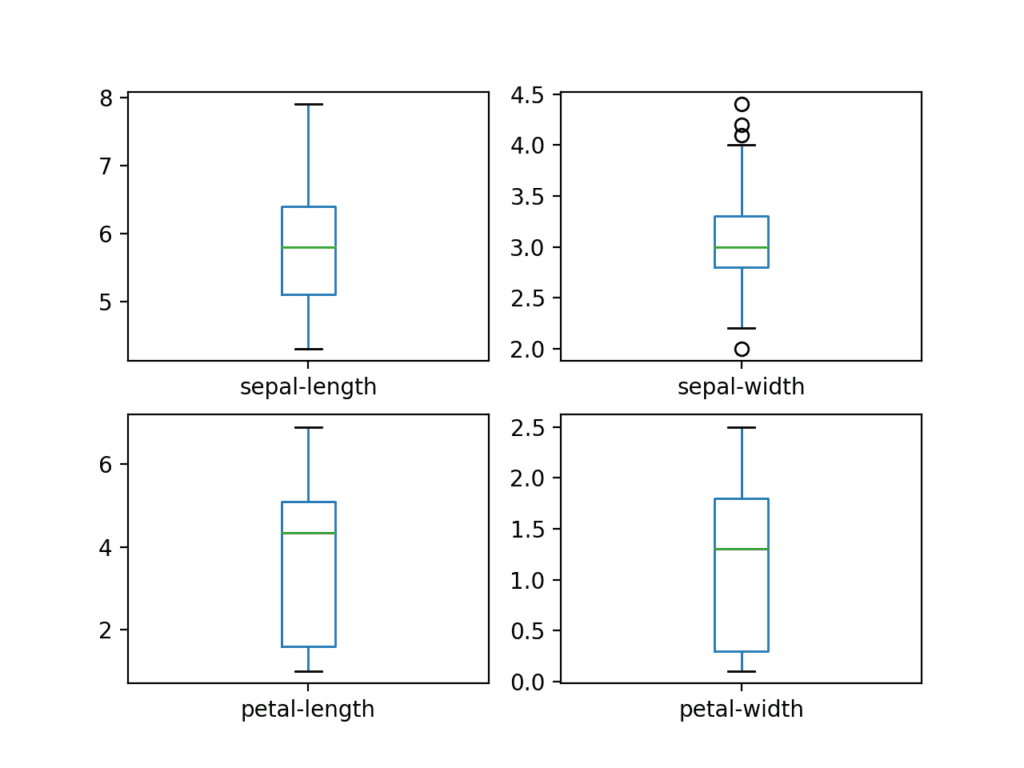
Box and Whisker Plots for Each Input Variable for the Iris Flowers Dataset
We can also create a histogram of each input variable to get an idea of the distribution.
1 2 3 4 | ... # histograms dataset.hist() plt.show() |
It looks like perhaps two of the input variables have a Gaussian distribution. This is useful to note as we can use algorithms that can exploit this assumption.
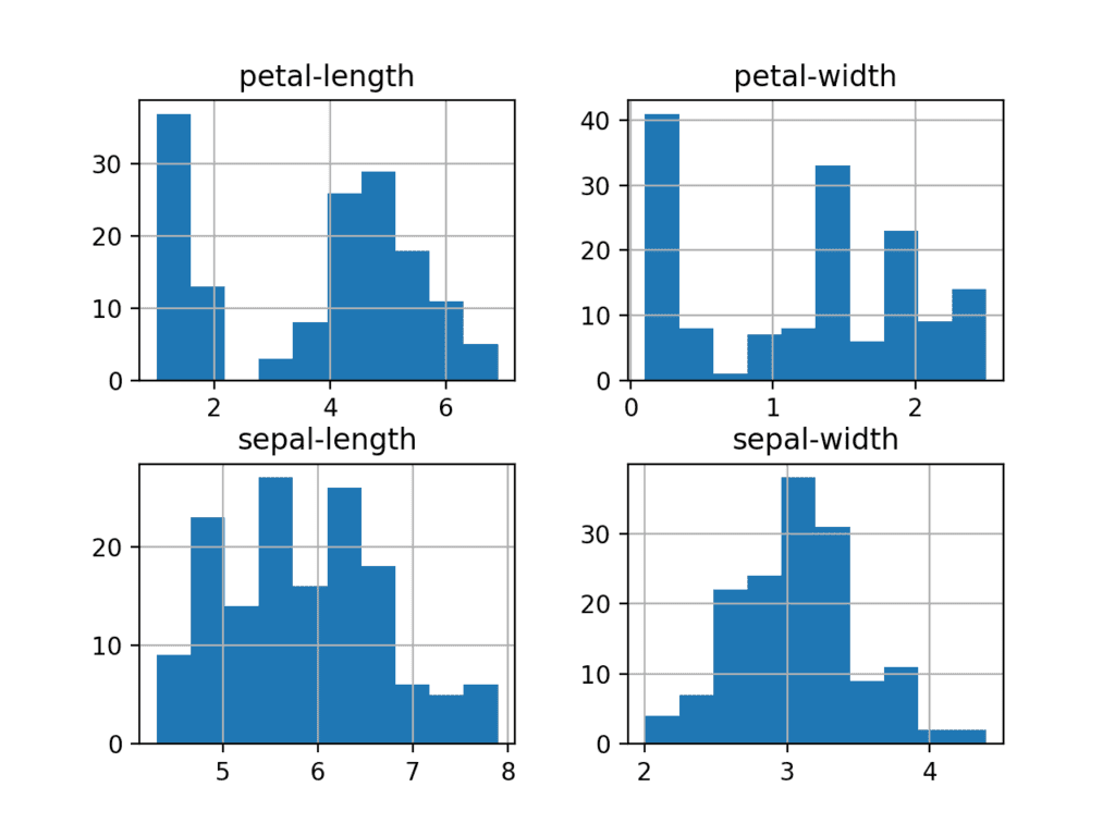
Histogram Plots for Each Input Variable for the Iris Flowers Dataset
4.2 Multivariate Plots
Now we can look at the interactions between the variables.
First, let’s look at scatterplots of all pairs of attributes. This can be helpful to spot structured relationships between input variables.
1 2 3 4 | ... # scatter plot matrix scatter_matrix(dataset) plt.show() |
Note the diagonal grouping of some pairs of attributes. This suggests a high correlation and a predictable relationship.
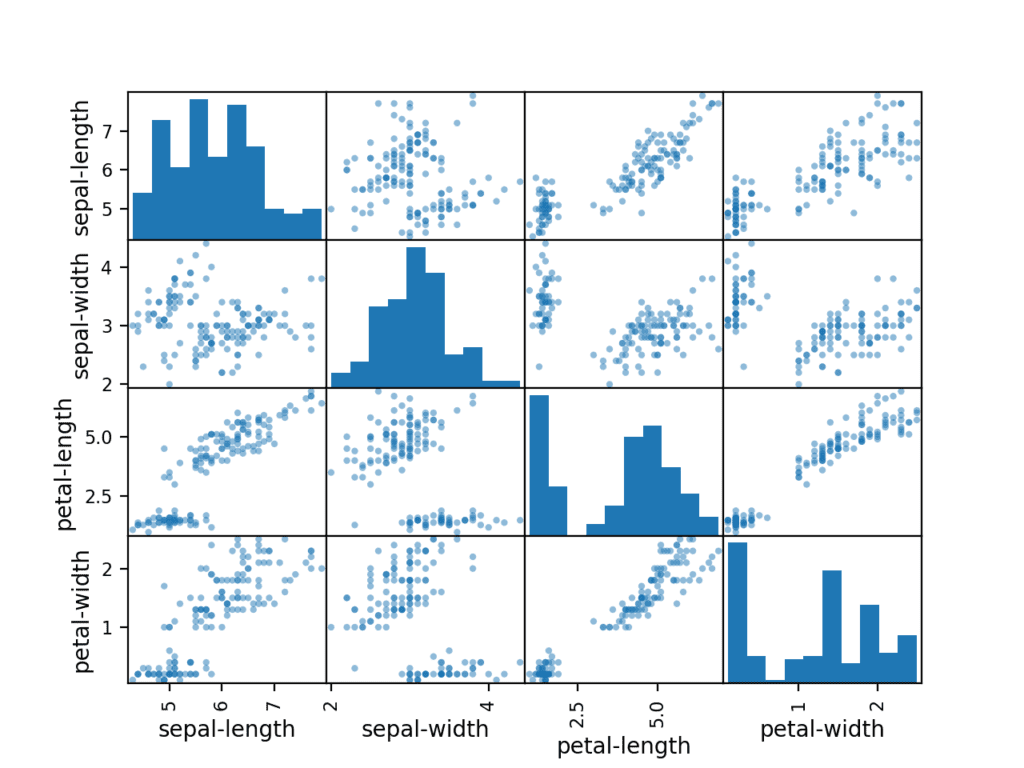
Scatter Matrix Plot for Each Input Variable for the Iris Flowers Dataset
4.3 Complete Example
For reference, we can tie all of the previous elements together into a single script.
The complete example is listed below.
1 2 3 4 5 6 7 8 9 10 11 12 13 14 15 16 17 | # visualize the data from pandas import read_csv from pandas.plotting import scatter_matrix from matplotlib import pyplot as plt # Load dataset url = "https://raw.githubusercontent.com/jbrownlee/Datasets/master/iris.csv" names = ['sepal-length', 'sepal-width', 'petal-length', 'petal-width', 'class'] dataset = read_csv(url, names=names) # box and whisker plots dataset.plot(kind='box', subplots=True, layout=(2,2), sharex=False, sharey=False) plt.show() # histograms dataset.hist() plt.show() # scatter plot matrix scatter_matrix(dataset) plt.show() |
5. Evaluate Some Algorithms
Now it is time to create some models of the data and estimate their accuracy on unseen data.
Here is what we are going to cover in this step:
- Separate out a validation dataset.
- Set-up the test harness to use 10-fold cross validation.
- Build multiple different models to predict species from flower measurements
- Select the best model.
5.1 Create a Validation Dataset
We need to know that the model we created is good.
Later, we will use statistical methods to estimate the accuracy of the models that we create on unseen data. We also want a more concrete estimate of the accuracy of the best model on unseen data by evaluating it on actual unseen data.
That is, we are going to hold back some data that the algorithms will not get to see and we will use this data to get a second and independent idea of how accurate the best model might actually be.
We will split the loaded dataset into two, 80% of which we will use to train, evaluate and select among our models, and 20% that we will hold back as a validation dataset.
1 2 3 4 5 6 | ... # Split-out validation dataset array = dataset.values X = array[:,0:4] y = array[:,4] X_train, X_validation, Y_train, Y_validation = train_test_split(X, y, test_size=0.20, random_state=1) |
You now have training data in the X_train and Y_train for preparing models and a X_validation and Y_validation sets that we can use later.
Notice that we used a python slice to select the columns in the NumPy array. If this is new to you, you might want to check-out this post:
5.2 Test Harness
We will use stratified 10-fold cross validation to estimate model accuracy.
This will split our dataset into 10 parts, train on 9 and test on 1 and repeat for all combinations of train-test splits.
Stratified means that each fold or split of the dataset will aim to have the same distribution of example by class as exist in the whole training dataset.
For more on the k-fold cross-validation technique, see the tutorial:
We set the random seed via the random_state argument to a fixed number to ensure that each algorithm is evaluated on the same splits of the training dataset.
The specific random seed does not matter, learn more about pseudorandom number generators here:
We are using the metric of ‘accuracy‘ to evaluate models.
This is a ratio of the number of correctly predicted instances divided by the total number of instances in the dataset multiplied by 100 to give a percentage (e.g. 95% accurate). We will be using the scoring variable when we run build and evaluate each model next.
5.3 Build Models
We don’t know which algorithms would be good on this problem or what configurations to use.
We get an idea from the plots that some of the classes are partially linearly separable in some dimensions, so we are expecting generally good results.
Let’s test 6 different algorithms:
- Logistic Regression (LR)
- Linear Discriminant Analysis (LDA)
- K-Nearest Neighbors (KNN).
- Classification and Regression Trees (CART).
- Gaussian Naive Bayes (NB).
- Support Vector Machines (SVM).
This is a good mixture of simple linear (LR and LDA), nonlinear (KNN, CART, NB and SVM) algorithms.
Let’s build and evaluate our models:
1 2 3 4 5 6 7 8 9 10 11 12 13 14 15 16 17 18 | ... # Spot Check Algorithms models = [] models.append(('LR', LogisticRegression(solver='liblinear', multi_class='ovr'))) models.append(('LDA', LinearDiscriminantAnalysis())) models.append(('KNN', KNeighborsClassifier())) models.append(('CART', DecisionTreeClassifier())) models.append(('NB', GaussianNB())) models.append(('SVM', SVC(gamma='auto'))) # evaluate each model in turn results = [] names = [] for name, model in models: kfold = StratifiedKFold(n_splits=10, random_state=1, shuffle=True) cv_results = cross_val_score(model, X_train, Y_train, cv=kfold, scoring='accuracy') results.append(cv_results) names.append(name) print('%s: %f (%f)' % (name, cv_results.mean(), cv_results.std())) |
5.4 Select Best Model
We now have 6 models and accuracy estimations for each. We need to compare the models to each other and select the most accurate.
Running the example above, we get the following raw results:
1 2 3 4 5 6 | LR: 0.960897 (0.052113) LDA: 0.973974 (0.040110) KNN: 0.957191 (0.043263) CART: 0.957191 (0.043263) NB: 0.948858 (0.056322) SVM: 0.983974 (0.032083) |
Note: Your results may vary given the stochastic nature of the algorithm or evaluation procedure, or differences in numerical precision. Consider running the example a few times and compare the average outcome.
What scores did you get?
Post your results in the comments below.
In this case, we can see that it looks like Support Vector Machines (SVM) has the largest estimated accuracy score at about 0.98 or 98%.
We can also create a plot of the model evaluation results and compare the spread and the mean accuracy of each model. There is a population of accuracy measures for each algorithm because each algorithm was evaluated 10 times (via 10 fold-cross validation).
A useful way to compare the samples of results for each algorithm is to create a box and whisker plot for each distribution and compare the distributions.
1 2 3 4 5 | ... # Compare Algorithms plt.boxplot(results, labels=names) plt.title('Algorithm Comparison') plt.show() |
We can see that the box and whisker plots are squashed at the top of the range, with many evaluations achieving 100% accuracy, and some pushing down into the high 80% accuracies.
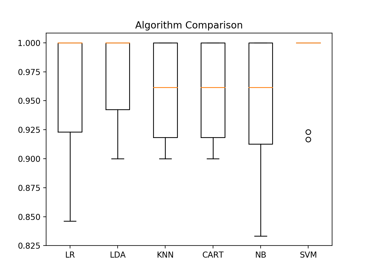
Box and Whisker Plot Comparing Machine Learning Algorithms on the Iris Flowers Dataset
5.5 Complete Example
For reference, we can tie all of the previous elements together into a single script.
The complete example is listed below.
1 2 3 4 5 6 7 8 9 10 11 12 13 14 15 16 17 18 19 20 21 22 23 24 25 26 27 28 29 30 31 32 33 34 35 36 37 38 39 40 41 42 | # compare algorithms from pandas import read_csv from matplotlib import pyplot as plt from sklearn.model_selection import train_test_split from sklearn.model_selection import cross_val_score from sklearn.model_selection import StratifiedKFold from sklearn.linear_model import LogisticRegression from sklearn.tree import DecisionTreeClassifier from sklearn.neighbors import KNeighborsClassifier from sklearn.discriminant_analysis import LinearDiscriminantAnalysis from sklearn.naive_bayes import GaussianNB from sklearn.svm import SVC # Load dataset url = "https://raw.githubusercontent.com/jbrownlee/Datasets/master/iris.csv" names = ['sepal-length', 'sepal-width', 'petal-length', 'petal-width', 'class'] dataset = read_csv(url, names=names) # Split-out validation dataset array = dataset.values X = array[:,0:4] y = array[:,4] X_train, X_validation, Y_train, Y_validation = train_test_split(X, y, test_size=0.20, random_state=1, shuffle=True) # Spot Check Algorithms models = [] models.append(('LR', LogisticRegression(solver='liblinear', multi_class='ovr'))) models.append(('LDA', LinearDiscriminantAnalysis())) models.append(('KNN', KNeighborsClassifier())) models.append(('CART', DecisionTreeClassifier())) models.append(('NB', GaussianNB())) models.append(('SVM', SVC(gamma='auto'))) # evaluate each model in turn results = [] names = [] for name, model in models: kfold = StratifiedKFold(n_splits=10, random_state=1, shuffle=True) cv_results = cross_val_score(model, X_train, Y_train, cv=kfold, scoring='accuracy') results.append(cv_results) names.append(name) print('%s: %f (%f)' % (name, cv_results.mean(), cv_results.std())) # Compare Algorithms plt.boxplot(results, labels=names) plt.title('Algorithm Comparison') plt.show() |
6. Make Predictions
We must choose an algorithm to use to make predictions.
The results in the previous section suggest that the SVM was perhaps the most accurate model. We will use this model as our final model.
Now we want to get an idea of the accuracy of the model on our validation set.
This will give us an independent final check on the accuracy of the best model. It is valuable to keep a validation set just in case you made a slip during training, such as overfitting to the training set or a data leak. Both of these issues will result in an overly optimistic result.
6.1 Make Predictions
We can fit the model on the entire training dataset and make predictions on the validation dataset.
1 2 3 4 5 | ... # Make predictions on validation dataset model = SVC(gamma='auto') model.fit(X_train, Y_train) predictions = model.predict(X_validation) |
You might also like to make predictions for single rows of data. For examples on how to do that, see the tutorial:
You might also like to save the model to file and load it later to make predictions on new data. For examples on how to do this, see the tutorial:
6.2 Evaluate Predictions
We can evaluate the predictions by comparing them to the expected results in the validation set, then calculate classification accuracy, as well as a confusion matrix and a classification report.
1 2 3 4 5 | .... # Evaluate predictions print(accuracy_score(Y_validation, predictions)) print(confusion_matrix(Y_validation, predictions)) print(classification_report(Y_validation, predictions)) |
We can see that the accuracy is 0.966 or about 96% on the hold out dataset.
The confusion matrix provides an indication of the errors made.
Finally, the classification report provides a breakdown of each class by precision, recall, f1-score and support showing excellent results (granted the validation dataset was small).
1 2 3 4 5 6 7 8 9 10 11 12 13 | 0.9666666666666667 [[11 0 0] [ 0 12 1] [ 0 0 6]] precision recall f1-score support Iris-setosa 1.00 1.00 1.00 11 Iris-versicolor 1.00 0.92 0.96 13 Iris-virginica 0.86 1.00 0.92 6 accuracy 0.97 30 macro avg 0.95 0.97 0.96 30 weighted avg 0.97 0.97 0.97 30 |
6.3 Complete Example
For reference, we can tie all of the previous elements together into a single script.
The complete example is listed below.
1 2 3 4 5 6 7 8 9 10 11 12 13 14 15 16 17 18 19 20 21 22 23 24 | # make predictions from pandas import read_csv from sklearn.model_selection import train_test_split from sklearn.metrics import classification_report from sklearn.metrics import confusion_matrix from sklearn.metrics import accuracy_score from sklearn.svm import SVC # Load dataset url = "https://raw.githubusercontent.com/jbrownlee/Datasets/master/iris.csv" names = ['sepal-length', 'sepal-width', 'petal-length', 'petal-width', 'class'] dataset = read_csv(url, names=names) # Split-out validation dataset array = dataset.values X = array[:,0:4] y = array[:,4] X_train, X_validation, Y_train, Y_validation = train_test_split(X, y, test_size=0.20, random_state=1) # Make predictions on validation dataset model = SVC(gamma='auto') model.fit(X_train, Y_train) predictions = model.predict(X_validation) # Evaluate predictions print(accuracy_score(Y_validation, predictions)) print(confusion_matrix(Y_validation, predictions)) print(classification_report(Y_validation, predictions)) |
You Can Do Machine Learning in Python
Work through the tutorial above. It will take you 5-to-10 minutes, max!
You do not need to understand everything. (at least not right now) Your goal is to run through the tutorial end-to-end and get a result. You do not need to understand everything on the first pass. List down your questions as you go. Make heavy use of the help(“FunctionName”) help syntax in Python to learn about all of the functions that you’re using.
You do not need to know how the algorithms work. It is important to know about the limitations and how to configure machine learning algorithms. But learning about algorithms can come later. You need to build up this algorithm knowledge slowly over a long period of time. Today, start off by getting comfortable with the platform.
You do not need to be a Python programmer. The syntax of the Python language can be intuitive if you are new to it. Just like other languages, focus on function calls (e.g. function()) and assignments (e.g. a = “b”). This will get you most of the way. You are a developer, you know how to pick up the basics of a language real fast. Just get started and dive into the details later.
You do not need to be a machine learning expert. You can learn about the benefits and limitations of various algorithms later, and there are plenty of posts that you can read later to brush up on the steps of a machine learning project and the importance of evaluating accuracy using cross validation.
What about other steps in a machine learning project. We did not cover all of the steps in a machine learning project because this is your first project and we need to focus on the key steps. Namely, loading data, looking at the data, evaluating some algorithms and making some predictions. In later tutorials we can look at other data preparation and result improvement tasks.
Summary
In this post, you discovered step-by-step how to complete your first machine learning project in Python.
You discovered that completing a small end-to-end project from loading the data to making predictions is the best way to get familiar with a new platform.
Your Next Step
Do you work through the tutorial?
- Work through the above tutorial.
- List any questions you have.
- Search-for or research the answers.
- Remember, you can use the help(“FunctionName”) in Python to get help on any function.
Do you have a question?
Post it in the comments below.


No comments:
Post a Comment