Outliers are unique in that they often don’t play by the rules. These data points, which significantly differ from the rest, can skew your analyses and make your predictive models less accurate. Although detecting outliers is critical, there is no universally agreed-upon method for doing so. While some advanced techniques like machine learning offer solutions, in this post, we will focus on the foundational Data Science methods that have been in use for decades.
Let’s get started.
Overview
This post is divided into three parts; they are:
- Understanding Outliers and Their Impact
- Traditional Methods for Outlier Detection
- Detecting Outliers in the Ames Dataset
Understanding Outliers and Their Impact
Outliers can emerge for a variety of reasons, from data entry errors to genuine anomalies. Their presence can be attributed to factors like:
- Measurement errors
- Data processing errors
- Genuine extreme observations
Understanding the source of an outlier is crucial for determining whether to keep, modify, or discard it. The impact of outliers on statistical analyses can be profound. They can change the results of data visualizations, central tendency measurements, and other statistical tests. Outliers can also influence the assumptions of normality, linearity, and homoscedasticity in a dataset, leading to unreliable and spurious conclusions.
Traditional Methods for Outlier Detection
In the realm of Data Science, several classical methods exist for detecting outliers. These can be broadly categorized into:
- Visual methods: Plots and graphs, such as scatter plots, box plots, and histograms, provide an intuitive feel of the data distribution and any extreme values.
- Statistical methods: Techniques like the Z-score, IQR (Interquartile Range), and the modified Z-score are mathematical methods used to define outliers based on data distribution.
- Probabilistic and statistical models: These leverage the probability distribution of data, such as the Gaussian distribution, to detect unlikely observations.
It’s essential to understand that the choice of method often depends on the nature of your dataset and the specific problem at hand.
Detecting Outliers in the Ames Dataset
In this section, you’ll dive into the practical application of detecting outliers using the Ames Housing Dataset. Specifically, you’ll explore three features: Lot Area, Sales Price, and Total Rooms Above Ground.
Visual Inspection
Visual methods are a quick and intuitive way to identify outliers. Let’s start with box plots for your chosen features.
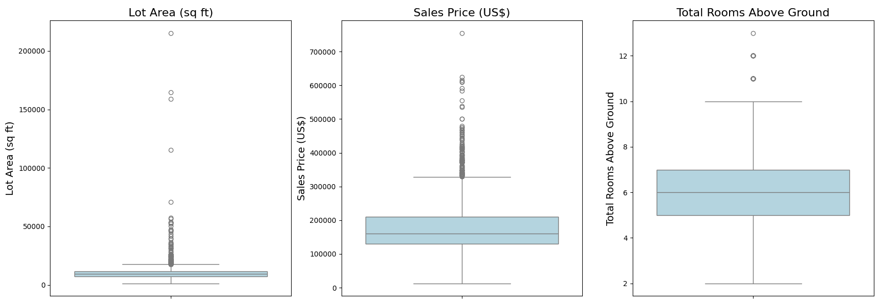
These plots provide immediate insights into potential outliers in your data. The dots you see beyond the whiskers represent data points that are considered outliers, lying outside 1.5 times the Interquartile Range (IQR) from the first and third quartiles. For instance, you might notice properties with exceptionally large lot areas or homes with a large number of rooms above ground.
Statistical Methods: IQR
The dots in the box plots above are greater than 1.5 times the Interquartile Range (IQR) from the third quartiles. It is a robust method to quantitatively identify outliers. You can precisely find and count these dots from the pandas DataFrame without the box plot:
This prints:
In your analysis of the Ames Housing Dataset using the Interquartile Range (IQR) method, you identified 113 outliers in the “Lot Area” feature, 116 outliers in the “Sales Price” feature, and 35 outliers for the “Total Rooms Above Ground” feature. These outliers are visually represented as dots beyond the whiskers in the box plots. The whiskers of the box plots typically extend up to 1.5 times the IQR from the first and third quartiles, and data points beyond these whiskers are considered outliers. This is just one definition of outliers. Such values should be further investigated or treated appropriately in subsequent analyses.
Probabilistic and Statistical Models
The natural distribution of data can sometimes help you identify outliers. One of the most common assumptions about data distribution is that it follows a Gaussian (or normal) distribution. In a perfectly Gaussian distribution, about 68% of the data lies within one standard deviation from the mean, 95% within two standard deviations, and 99.7% within three standard deviations. Data points that fall far away from the mean (typically beyond three standard deviations) can be considered outliers.
This method is particularly effective when the dataset is large and is believed to be normally distributed. Let’s apply this technique to your Ames Housing Dataset and see what you find.
This shows these charts of distribution: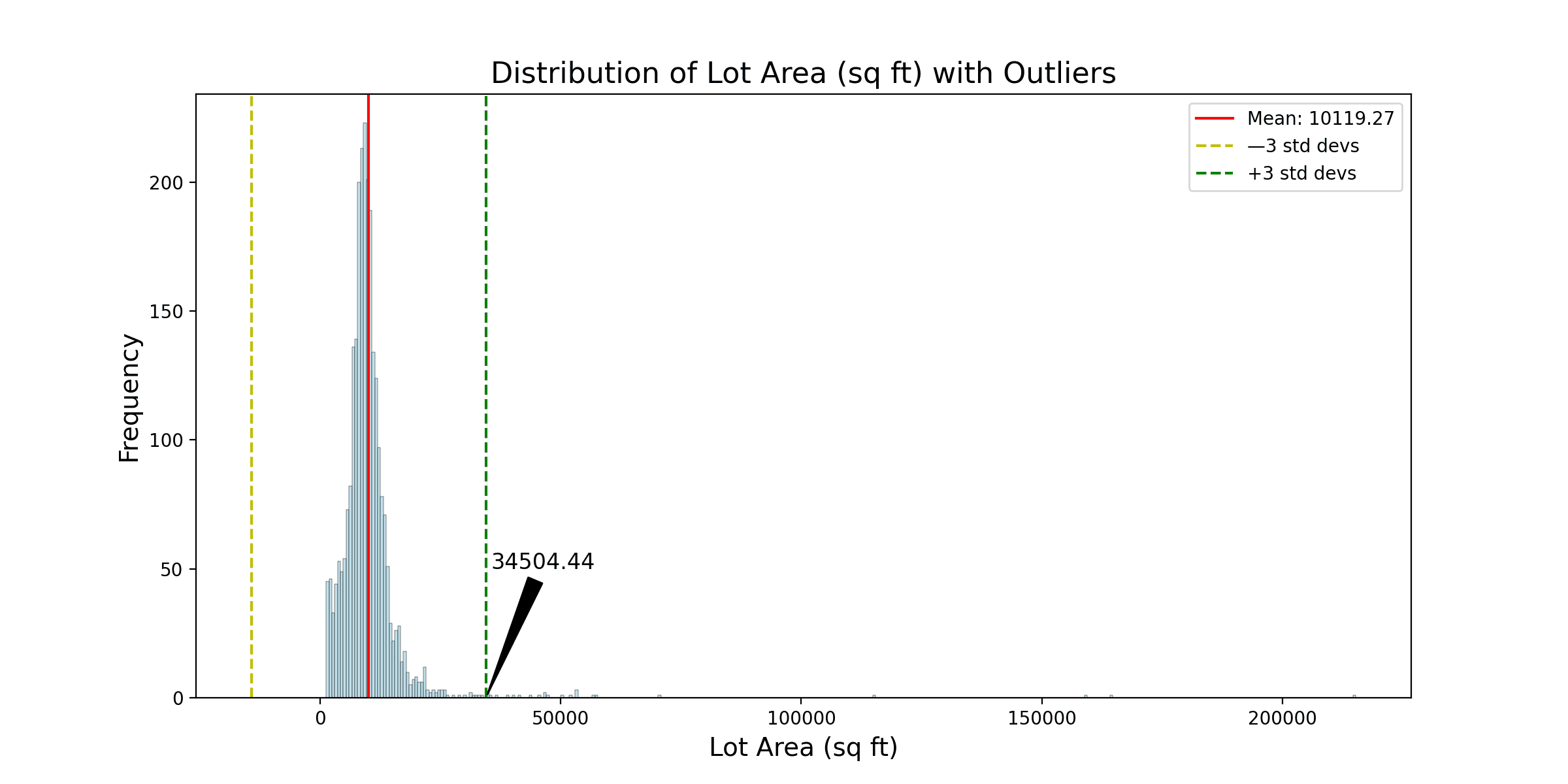
 Then it prints the following:
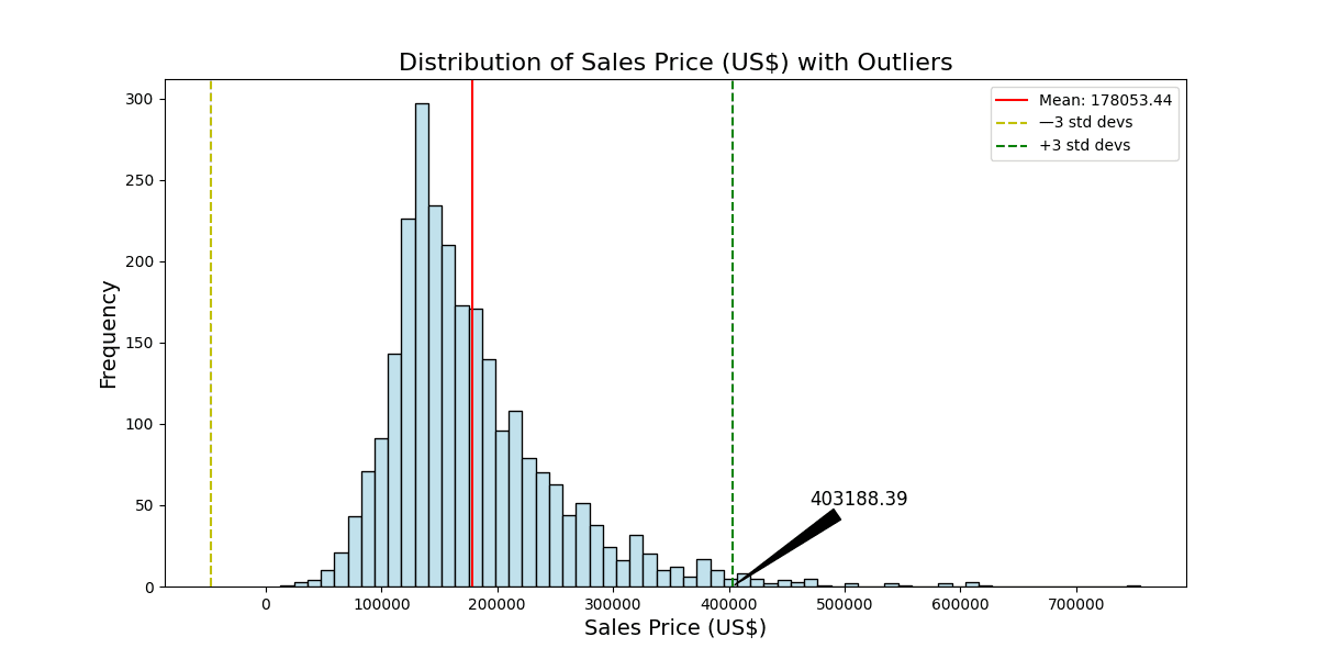
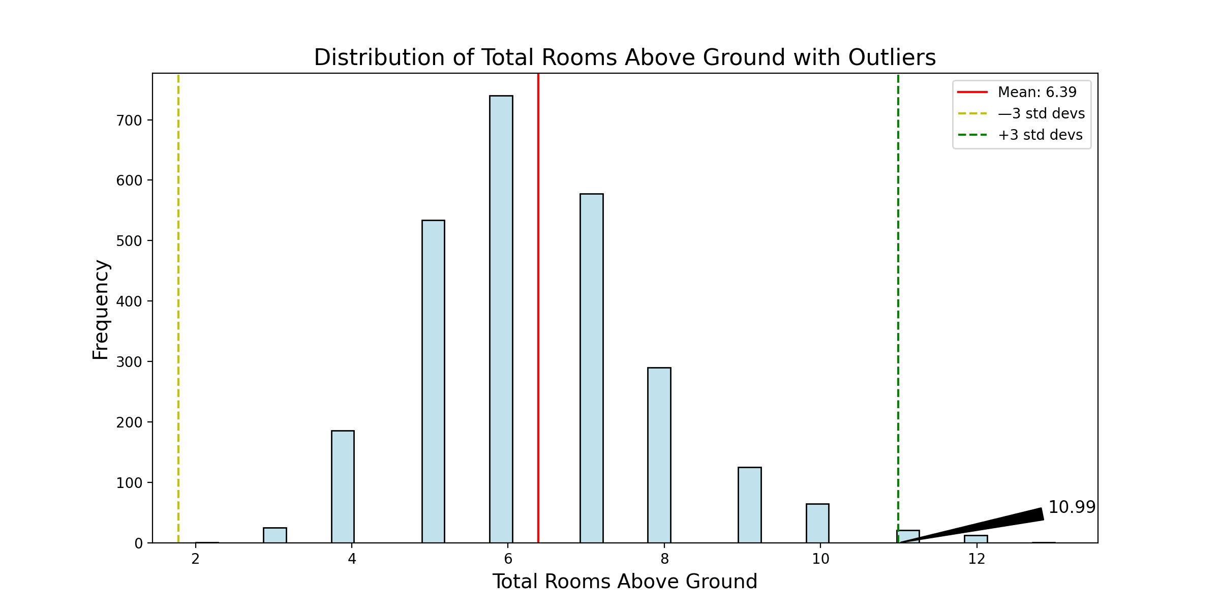
Upon applying the Gaussian model for outlier detection, you observed that there are outliers in the “Lot Area,” “Sales Price,” and “Total Rooms Above Ground” features. These outliers are identified based on the upper threshold of three standard deviations from the mean:
- Lot Area: Any observation with a lot area larger than 34,505.44 square feet is considered an outlier. You found 24 such outliers in the dataset.
- Sales Price: Any observation above US$403,188.39 is considered an outlier. Your analysis revealed 42 outliers in the “Sales Price” feature.
- Total Rooms Above Ground: Observations with more than 10.99 rooms above ground are considered outliers. You identified 35 outliers using this criterion.
The number of outliers is different because the definition of outliers is different. These figures differ from your earlier IQR method, emphasizing the importance of utilizing multiple techniques for a more comprehensive understanding. The visualizations accentuate these outliers, allowing for a clear distinction from the main distribution of the data. Such discrepancies underscore the necessity of domain expertise and context when deciding on the best approach for outlier management.
To enhance your understanding and facilitate further analysis, it’s valuable to compile a comprehensive list of identified outliers. This list provides a clear overview of the specific data points that deviate significantly from the norm. In the following section, you’ll illustrate how to systematically organize and list these outliers into a DataFrame for each feature: “Lot Area,” “Sales Price,” and “Total Rooms Above Ground.” This tabulated format allows for easy inspection and potential actions, such as further investigation or targeted data treatment.
Let’s explore the approach that accomplishes this task.
Now, before you unveil the results, it’s essential to note that the code snippet allows for user customization. By adjusting the parameter num_rows, you have the flexibility to define the number of rows you want to see in each DataFrame. In the example shared earlier, you used num_rows=7 for a concise display, but the default setting is num_rows=None, which prints the entire DataFrame. Feel free to tailor this parameter to suit your preferences and the specific requirements of your analysis.
In this exploration of probabilistic and statistical models for outlier detection, you focused on the Gaussian model applied to the Ames Housing Dataset, specifically utilizing a threshold of three standard deviations. By leveraging the insights provided by visualizations and statistical methods, you identified outliers and demonstrated their listing in a customizable DataFrame.
Further Reading
Resources
Summary
Outliers, stemming from diverse causes, significantly impact statistical analyses. Recognizing their origins is crucial as they can distort visualizations, central tendency measures, and statistical tests. Classical Data Science methods for outlier detection encompass visual, statistical, and probabilistic approaches, with the choice dependent on dataset nature and specific problems.
Application of these methods on the Ames Housing Dataset, focusing on Lot Area, Sales Price, and Total Rooms Above Ground, revealed insights. Visual methods like box plots provided quick outlier identification. The Interquartile Range (IQR) method quantified outliers, revealing 113, 116, and 35 outliers for Lot Area, Sales Price, and Total Rooms Above Ground. Probabilistic models, particularly the Gaussian model with three standard deviations, found 24, 42, and 35 outliers in the respective features.
These results underscore the need for a multifaceted approach to outlier detection. Beyond identification, systematically organizing and listing outliers in tabulated DataFrames facilitates in-depth inspection. Customizability, demonstrated by the num_rows parameter, ensures flexibility in presenting tailored results. In conclusion, this exploration enhances understanding and provides practical guidance for managing outliers in real-world datasets.
Specifically, you learned:
- The significance of outliers and their potential impact on data analyses.
- Various traditional methods are used in Data Science for outlier detection.
- How to apply these methods in a real-world dataset, using the Ames Housing Dataset as an example.
- Systematic organization and listing of identified outliers into customizable DataFrames for detailed inspection and further analysis.
Do you have any questions? Please ask your questions in the comments below, and I will do my best to answer.


No comments:
Post a Comment