You may have observations at the wrong frequency.
Maybe they are too granular or not granular enough. The Pandas library in Python provides the capability to change the frequency of your time series data.
In this tutorial, you will discover how to use Pandas in Python to both increase and decrease the sampling frequency of time series data.
After completing this tutorial, you will know:
- About time series resampling, the two types of resampling, and the 2 main reasons why you need to use them.
- How to use Pandas to upsample time series data to a higher frequency and interpolate the new observations.
- How to use Pandas to downsample time series data to a lower frequency and summarize the higher frequency observations.
Kick-start your project with my new book Time Series Forecasting With Python, including step-by-step tutorials and the Python source code files for all examples.
Let’s get started.
- Update Dec/2016: Fixed definitions of upsample and downsample.
- Updated Apr/2019: Updated the link to dataset.

How To Resample and Interpolate Your Time Series Data With Python
Photo by sung ming whang, some rights reserved.
Resampling
Resampling involves changing the frequency of your time series observations.
Two types of resampling are:
- Upsampling: Where you increase the frequency of the samples, such as from minutes to seconds.
- Downsampling: Where you decrease the frequency of the samples, such as from days to months.
In both cases, data must be invented.
In the case of upsampling, care may be needed in determining how the fine-grained observations are calculated using interpolation. In the case of downsampling, care may be needed in selecting the summary statistics used to calculate the new aggregated values.
There are perhaps two main reasons why you may be interested in resampling your time series data:
- Problem Framing: Resampling may be required if your data is not available at the same frequency that you want to make predictions.
- Feature Engineering: Resampling can also be used to provide additional structure or insight into the learning problem for supervised learning models.
There is a lot of overlap between these two cases.
For example, you may have daily data and want to predict a monthly problem. You could use the daily data directly or you could downsample it to monthly data and develop your model.
A feature engineering perspective may use observations and summaries of observations from both time scales and more in developing a model.
Let’s make resampling more concrete by looking at a real dataset and some examples.
Stop learning Time Series Forecasting the slow way!
Take my free 7-day email course and discover how to get started (with sample code).
Click to sign-up and also get a free PDF Ebook version of the course.
Shampoo Sales Dataset
This dataset describes the monthly number of sales of shampoo over a 3 year period.
The units are a sales count and there are 36 observations. The original dataset is credited to Makridakis, Wheelwright, and Hyndman (1998).
Below is a sample of the first 5 rows of data, including the header row.
Below is a plot of the entire dataset.
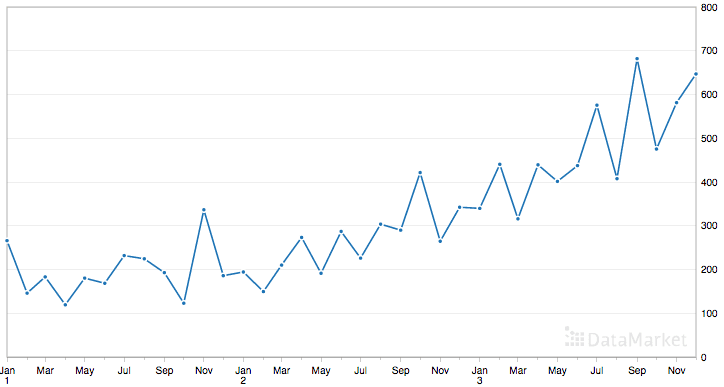
Shampoo Sales Dataset
The dataset shows an increasing trend and possibly some seasonal components.
Load the Shampoo Sales Dataset
Download the dataset and place it in the current working directory with the filename “shampoo-sales.csv“.
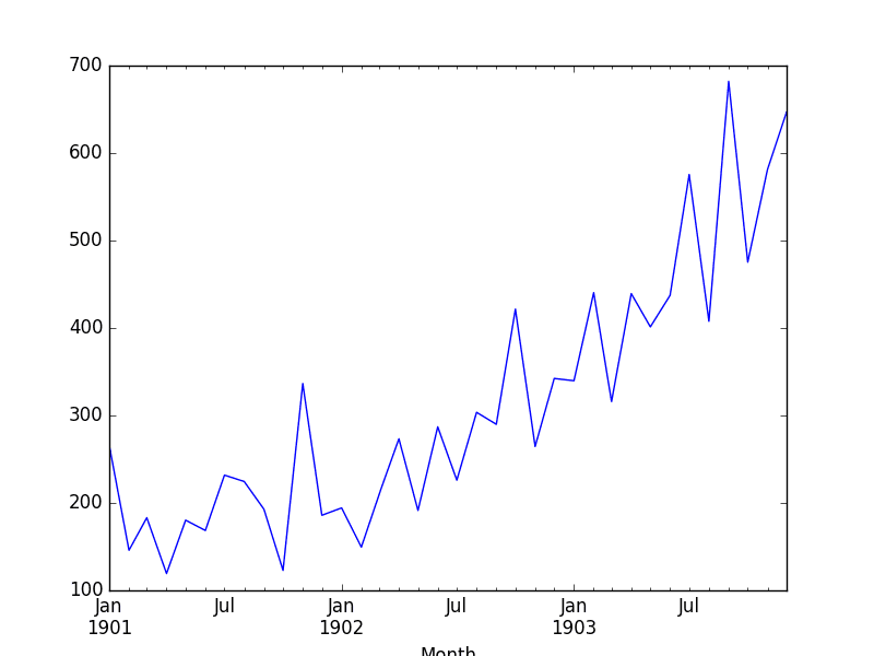
The timestamps in the dataset do not have an absolute year, but do have a month. We can write a custom date parsing function to load this dataset and pick an arbitrary year, such as 1900, to baseline the years from.
Below is a snippet of code to load the Shampoo Sales dataset using the custom date parsing function from read_csv().
Running this example loads the dataset and prints the first 5 rows. This shows the correct handling of the dates, baselined from 1900.
We also get a plot of the dataset, showing the rising trend in sales from month to month.

Plot of the Shampoo Sales Dataset
Upsample Shampoo Sales
The observations in the Shampoo Sales are monthly.
Imagine we wanted daily sales information. We would have to upsample the frequency from monthly to daily and use an interpolation scheme to fill in the new daily frequency.
The Pandas library provides a function called resample() on the Series and DataFrame objects. This can be used to group records when downsampling and making space for new observations when upsampling.
We can use this function to transform our monthly dataset into a daily dataset by calling resampling and specifying the preferred frequency of calendar day frequency or “D”.
Pandas is clever and you could just as easily specify the frequency as “1D” or even something domain specific, such as “5D.” See the further reading section at the end of the tutorial for the list of aliases that you can use.
Running this example prints the first 32 rows of the upsampled dataset, showing each day of January and the first day of February.
We can see that the resample() function has created the rows by putting NaN values in the new values. We can see we still have the sales volume on the first of January and February from the original data.
Next, we can interpolate the missing values at this new frequency.
The Series Pandas object provides an interpolate() function to interpolate missing values, and there is a nice selection of simple and more complex interpolation functions. You may have domain knowledge to help choose how values are to be interpolated.
A good starting point is to use a linear interpolation. This draws a straight line between available data, in this case on the first of the month, and fills in values at the chosen frequency from this line.
Running this example, we can see interpolated values.
Looking at a line plot, we see no difference from plotting the original data as the plot already interpolated the values between points to draw the line.
Shampoo Sales Interpolated Linear
Another common interpolation method is to use a polynomial or a spline to connect the values.
This creates more curves and can look more natural on many datasets. Using a spline interpolation requires you specify the order (number of terms in the polynomial); in this case, an order of 2 is just fine.
Running the example, we can first review the raw interpolated values.
Reviewing the line plot, we can see more natural curves on the interpolated values.

Shampoo Sales Interpolated Spline
Generally, interpolation is a useful tool when you have missing observations.
Next, we will consider resampling in the other direction and decreasing the frequency of observations.
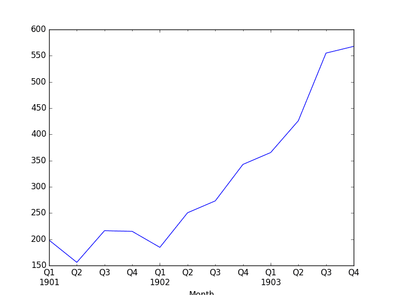
Downsample Shampoo Sales
The sales data is monthly, but perhaps we would prefer the data to be quarterly.
The year can be divided into 4 business quarters, 3 months a piece.
Instead of creating new rows between existing observations, the resample() function in Pandas will group all observations by the new frequency.
We could use an alias like “3M” to create groups of 3 months, but this might have trouble if our observations did not start in January, April, July, or October. Pandas does have a quarter-aware alias of “Q” that we can use for this purpose.
We must now decide how to create a new quarterly value from each group of 3 records. A good starting point is to calculate the average monthly sales numbers for the quarter. For this, we can use the mean() function.
Putting this all together, we get the following code example.
Running the example prints the first 5 rows of the quarterly data.
We also plot the quarterly data, showing Q1-Q4 across the 3 years of original observations.
Shampoo Sales Downsampled Quarterly
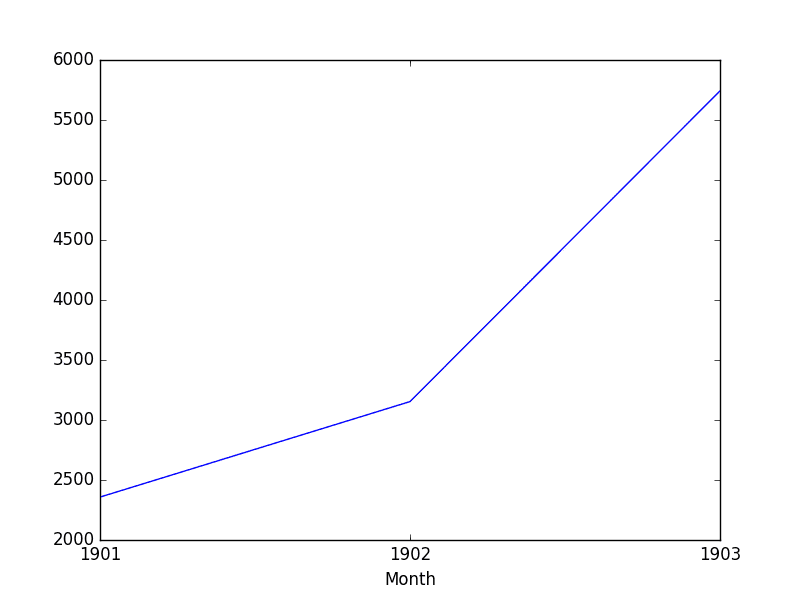
Perhaps we want to go further and turn the monthly data into yearly data, and perhaps later use that to model the following year.
We can downsample the data using the alias “A” for year-end frequency and this time use sum to calculate the total sales each year.
Running the example shows the 3 records for the 3 years of observations.
We also get a plot, correctly showing the year along the x-axis and the total number of sales per year along the y-axis.
Shampoo Sales Downsampled Yearly Sum
Further Reading
This section provides links and further reading for the Pandas functions used in this tutorial.
- pandas.Series.resample API documentation for more on how to configure the resample() function.
- Pandas Time Series Resampling Examples for more general code examples.
- Pandas Offset Aliases used when resampling for all the built-in methods for changing the granularity of the data.
- pandas.Series.interpolate API documentation for more on how to configure the interpolate() function.
Summary
In this tutorial, you discovered how to resample your time series data using Pandas in Python.
Specifically, you learned:
- About time series resampling and the difference and reasons between downsampling and upsampling observation frequencies.
- How to upsample time series data using Pandas and how to use different interpolation schemes.
- How to downsample time series data using Pandas and how to summarize grouped data.
Do you have any questions about resampling or interpolating time series data or about this tutorial?
Ask your questions in the comments and I will do my best to answer them.